This section takes a less customary perspective on the investigation of a cemetery in GIS that will provide outputs based on attributes and different methods from those used in Section 7.1, where simple distribution plans were studied. The results achieved by computing spatial density can, however, easily be compared with the outcomes presented above on the distribution plans. Both approaches can be evaluated together in terms of the spatio-temporal development of the site.
Now the basic analytical unit is not a single grave, but a square cell belonging to a regular grid over the whole funerary area. This approach is perhaps slightly unconventional in the context of cemetery investigation, where individual grave/burial seems to be the most natural point of analysis, but it offers interesting new avenues of research.
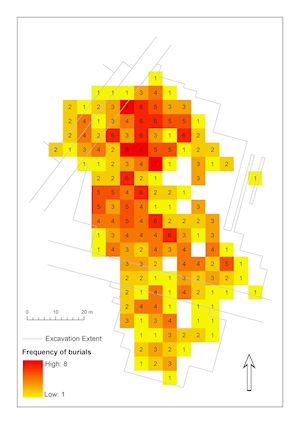
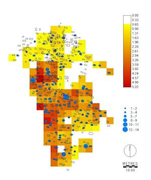
A brief explanation of the chosen grid parameters is necessary at this point. I have experimented with a variety of grid sizes, orientations and origins; the results obtained, however, were always in general agreement in their main outlines, which means that the patterns revealed are primarily a quality of the investigated data and not of the arbitrary analytical grid. The optimal spatial unit for most of the GIS raster procedures applied at Holešov seems to be a square of 5 x 5m. This size is not derived by any sophisticated algorithm; I simply created a series of outputs based on variable grid cell dimensions, starting from 1 x 1m and increasing the size of cells by 1m every time. Grids consisting of small cells produce many isolated (non-adjacent) squares that contain one or rarely more graves and the variability of observed values is reduced, which is less suitable for further processing. Going to the other extreme, a lower resolution of the grid would hide the details of patterns. When the plan of the site is overlaid with a grid of optimal parameters (5x5m), 158 squares (cells) containing from one to eight burials are obtained, the rest bearing zero value (Figure 10a). An important aspect of this grid resolution is that non-empty cells cover the whole funerary area more or less continuously and at the same time they provide a high number of comparable analytical units. The association of individual burials with a particular cell in the grid technically depends on the position of the central point (centroid) of each grave pit. As several graves possessed two individuals instead of the more usual single body, the actual number of buried individuals was ascribed to the cell value. The density of burial events across the geographical space can be easily computed this way and used for further reasoning.
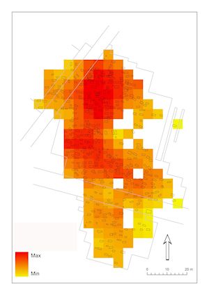
We can conclude that the density of burial events in different parts of the cemetery is not consistent (Figure 10a presents simple counts of burials in 5 x 5 m squares, Figure 10b shows a smoothed visualization of the same data, produced by a procedure described in Section 7.2.2). The northern part clearly demonstrates the highest intensity of use, the middle part shows lesser but still a fairly high frequency of burial, while the southern section and various marginal areas contain more sparsely distributed graves. The areas of higher burial density may possibly be explained either in terms of varying sizes of social units using different parts of the cemetery or – as I would prefer – as a function of time, during which a particular area was used for the disposal of the dead. In the zones with higher density, burials probably accumulated over a longer time period, assuming that average mortality rates remained more or less consistent. The dynamics of spatio-temporal development of this cemetery could combine at least two underlying mechanisms that may have operated simultaneously: 1) some of the deceased could be buried very near their relatives/ancestors, thus producing areas of high accumulations of graves, while 2) others presumably found their resting place at some distance along the edges of the earliest grave clusters. For some time they might appear spatially isolated and marginal but in the course of time they could become new foci of burial activity around which later graves started to cluster. The parallel processes of density increase and spatial expansion of the cemetery probably operated in a complex interplay dictated by the social relations and strategies of individuals and whole families or clans within the community that used the site as a burial ground.
If this model is correct, the northern and middle parts of the cemetery would contain burials from a wider time span than the south-eastern zone, where the density of burial events is low. Denser areas may therefore represent places where primary (earliest) burials were interred and additional graves surrounded them later on. This hypothesis is supported by the presence of Bell Beaker burials within these denser clusters. However, to exclude the possibility that such spatial arrangement developed by chance, the provisional model of spatial development (running basically from north to south) needs to be tested by mapping the densities of other variables – in this case of different categories of grave goods that accompany the burials. Their densities should be calculated and generalised in the same way as densities of the burials themselves (Figure 10a and 10b), using raster filtering functions in GIS.
Three important categories of artefacts will now be discussed; those made of chipped stone and those of copper alloys are expected to be chronologically indicative, although they frequently appear together in the burial assemblages and therefore their use must have been broadly contemporary. The third category discussed here is the rather enigmatic presence of animal - apparently cattle - ribs accompanying some burials. An interpretation of their function or symbolic meaning is unclear at the moment; we can nevertheless assume some strict rules commanding their role in the funerary ritual, as they seem to have been used almost exclusively in pairs of two, four or exceptionally six pieces (sometimes an odd number of ribs was recorded, but it seems to be the result of poor bone preservation). Attention will be paid to the dominance of these classes of artefacts in different parts of the site.
In the computed GIS outputs each cell is characterised by a colour, which corresponds to its filtered value. The final cell value thus stems from the absolute numbers of artefacts in the nine neighbouring cells (the cell in question and its eight immediate neighbours), comprising a kernel area of 15 x 15m. The 3 x 3 mean filter was chosen in order to take into account only local values and avoid averaging large areas. The task could also be accomplished by alternative methods of computing smooth interpolated surfaces but my present approach, based on the raster of a predefined resolution, allows for the generation of whole sets of raster images describing different attributes, which can then be easily compared and subjected to map algebra operations (this possibility is not followed up in this article; the outputs are used here only as aids for visual inspection). Because raster filters average values along the outer limits of sites where they produce distortive edge effects, I have applied a correction method to alleviate the problem as described elsewhere (Šmejda 2004, 62).
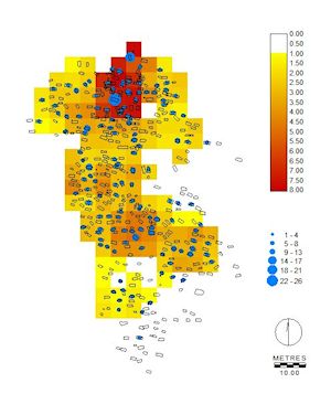
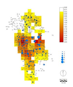
Two results of this procedure can now be investigated. The first one shows a major concentration of lithics (Figure 11a) located in the northernmost part of the site while the squares in the south-eastern edge of the cemetery lack chipped artefacts completely. This observation is in accordance with the identification of the earliest burials in the north and most of the late assemblages located at the opposite end of the cemetery (Ondráček 1972). The analysis of artefacts made of copper alloy seems to provide an inverted picture (Figure 11c). Metal finds are scarce in the north and relatively abundant in the middle and southern parts of the cemetery. Moreover, items made of copper alloy may be somewhat under-represented in the very south-eastern end of the site owing to a high frequency of 'robbed' graves in that part, a phenomenon typical for the Early Bronze Age and culminating towards the end of the period when it is known that metal objects were regularly removed from graves during their secondary re-opening (Stuchlík 1990; Neugebauer 1994; Sprenger 1999).
Cattle ribs also make a very clear spatial cluster of the highest filtered values, this time in the middle part of the cemetery (Figure 11b). Apparently, here they appear more frequently and in higher numbers than in squares located further north and south. All three spatial patterns just discussed can at certain levels express the chronology of the site. On the other hand there are possibly other factors that influence artefact distributions: for example, the social structure of the buried population both on vertical (in terms of social stratification) and horizontal (gender roles, specialisation) scale (Bátora 1991; Arnold and Wicker 2001).
In this selection of GIS analytical outputs presented in sections 7.2.1 and 7.2.2, we can see that different types of grave goods show different density patterns, despite the fact that they are usually present in every part of the cemetery. The non-homogeneous spatial density of their distribution is of course the significant factor, rather than their mere presence or absence. This approach proved that a raster analysis of this kind may be extremely useful even in funerary contexts, although traditionally it has been applied in studies operating at larger scales, such as landscape surveys or regional settlement studies (Neustupný 1998).
We can use the results as a foundation for building a chronological model of the site, supporting a hypothesis suggested by the excavator on the basis of the few highly disctinctive burial assemblages (Ondráček 1972). It seems that we can unambiguously detect opposing gradients of stone and copper artefact distributions that largely overlap but tend to concentrate in different parts of the site. Bearing in mind that we are dealing with the transitional period between the Stone and Bronze Ages, the spatial shift revealed here can most probably be directly connected to the shifts in technology and related symbolism used in the continuously developing burial practices.
I will conclude this section by a comparison between the density patterns of grave goods and the previously investigated density of burial events. Are they contributing to the same story? Most probably yes, although the patterns are neither completely identical nor contradictory. The area of the highest density of burials is subdivided into two parts. The northern part strikingly overlaps with the area of the highest accumulation of stone arrowheads, thus supporting the idea that it is the oldest core of the cemetery (because of the proliferation of stone implements and later accumulation of burials through time, though this continuity may not have lasted to the very end of site usage).
Another zone of high density of burials is located in the middle part of the cemetery, and this one partially overlaps with the highest concentration of animal ribs. It is not quite clear what separates the north and middle part of the site chronologically (if this occurs), because both areas include the earliest cultural phase – the Bell Beaker graves. It means these two parts may be broadly contemporary, having received interments over a considerable period of time, but they are still emphasising different elements of the ritual assemblage placed in the grave pit. While the north part is almost devoid of metal artefacts, but packed with chipped stone objects and containing only average numbers of animal ribs, the middle part shows cattle ribs in high quantities, average representation of flints and significant presence of copper ornaments that continues further south (where the densities of arrowheads and animal ribs decline in unison, supposedly because here the burials are relatively later, not following the final Stone Age funerary tradition so rigidly).
The spatial structures observed by the computation of densities thus provides a useful insight into the temporality of social use of space (Ingold 2010) within the slowly expanding area devoted to buried ancestors. Temporality in this sense does not equal to the relative chronology (though it naturally rests on the passage of time) but rather to the notion of how the small burial ground, once established, developed in the course of time, its different parts being adapted, redefined, abandoned and appropriated again. All in all it was linked to social groups in mutual co-evolution: the living used and continually transformed the funerary area as every single interment slightly changed the general context and particular relations between all graves, and on the other hand as the burial ground swallowed the members of local community one by one, it caused shifts and re-negotiations of social roles and individual statuses among the living.