For slope-dependent LCP calculations, a cost function is required that assigns costs to a path of given length and slope. The cost functions for walking and running humans differ (Minetti et al. 2002). Running was in fact an important way of transmitting messages in some cultures (Lay 1992, 20). If special paths were available for runners, these should be modelled in a different way from footpaths for walking. But in general, the messengers most probably used existing routes.
Several authors (e.g. Pingel 2009) point out that walking costs vary widely owing to different factors such as age, sex, health, fitness, body characteristics, and experience, but also weather conditions or wetness of the ground. For example, a study by Ainslie et al. (2002) measured the duration of a 12km hill walk involving 13 subjects ranging in age from 18 to 32. The slowest walker needed twice as much time as the fastest member of the study group. According to the authors of the study, the differences in velocity were mainly due to weather conditions. Imhof (1950, 217) points out that it does not make sense to try to be overly exact in measuring walking time because the time required depends on many factors.
These variations are irrelevant for LCP calculations if they involve a constant factor because, as mentioned in Section 4, multiplying the cost function by a positive constant does not change the LCP result. For example, Tobler (1993) suggests that his cost function is to be multiplied by 0.6 for off-path travel. So as long as the whole route is covered by off-path travel, the same cost function can be used as for walking on footpaths – if Tobler's assumption proves to be true. However, if a person walks as fast as a fit and well-trained soldier on level ground but is not able to maintain the speed of the soldier on a steep gradient, two different cost functions are required to model the slope-dependent velocity of these two persons appropriately. A plausible assumption is that the long-distance natural routes were created by well-trained people who travelled frequently, like the modern porters in the Himalayan region (Minetti et al. 2006), who at about 12 years of age already carry loads of about 35kg and stop as porters at the age of about 40–45 years. Therefore the cost function should be derived from walking data of young and well-trained people. Neither elite athletes (such as in Minetti et al. 2002) nor inexperienced hikers (such as in Kondo and Seino 2010) form the ideal test group for deriving an appropriate cost function.
Three ways of estimating the costs of walking or vehicle progress have been used in archaeological LCP studies: simple functions, time, and energy expenditure. The cost functions measuring time and energy expenditure were discussed in some detail by Herzog (2013a); for this reason, only a short overview for these two types of cost function is given in the corresponding sections (5.1.4.2 and 5.1.4.3) combined with some new aspects. But first the focus is on simple functions, which have been applied in several archaeological LCP studies.
A simple cost formula based on a physical model for ascending and descending slopes was developed by Bell and Lock (2000), and quite a few authors refer to this formula (van Leusen 2002, chapter 6, 6; Conolly and Lake 2006, 220, fig. 10.9; Chapman 2006, 108–9; Fábrega Álvarez and Parcero Oubiña 2007; Howey 2007; Bell et al. 2002).
Cost(ŝ) = tan(ŝ)/tan(1°)
where ŝ is slope in degree. This is the same as
Cost(s) = c * s
where s is per cent slope and c a constant factor. So in this approach, cost is proportional to per cent slope, i.e. the cost function Cost(s) = s will create the same LCP results. According to Conolly and Lake (2006, fig. 10.9, 220) this cost function assigns negative values to downhill slope values. This is problematic, as discussed in Section 4.
Basically the same function (multiplied by 0.1), but restricted to positive slope values including zero, was applied by Polla (2009) in her initial isotropic LCP analysis. In a second step, Polla tests several linear cost functions depending on positive slope, i.e. cost functions of the structure
Cost(s) = p*s + k
where s is per cent slope. The LCP results obtained with the parameters p=1 and k=1 are closest to the known route of a Roman road.
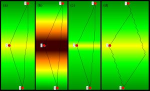
The main drawback of this sort of cost function is that it does not agree with the experience that small changes in slope are more relevant in terms of cost on a steep gradient than on fairly level ground. Owing to this property, LCPs calculated on the basis of this type of cost function ascend slopes directly, without switchbacks. For example, the LCP result of the cost function |s|+1 is independent of the slope of the artificial roof-shaped landscape (Figure 5a and 5b).
Van Leusen (2002, chapter 6, 6) presents the cost function applied by Hayden, which bears some similarity to the function initially used by Polla.
Cost(s) = s/10 if s > 0, Cost(s) = |s|/20 if s ≤ 0, with s = per cent slope
LCPs calculated on the basis of this cost function will also ascend or descend steep slopes without switchbacks, and therefore instead of (piecewise) linear functions simple quadratic functions are considered next. Llobera and Sluckin (2007) analyse hypothetical cost functions of the following form:
Cost(s) = a + b*s²
where s is mathematical slope, a and b are positive constants. As has been shown in Section 4, multiplying the cost function with a positive constant does not change the result of the LCP calculation. Therefore the following cost function is equivalent to the one presented above:
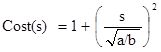
Llobera and Sluckin (2007) calculate the critical slope of this function, and the result is √(a/b). This means that a symmetric quadratic cost function can be easily constructed for a given critical slope š:
Cost(s) = 1 + (s / š)²
where š and s are per cent slope values (or both are mathematical slope values). This quadratic cost function is symmetric and therefore, it is only appropriate if bi-directional routes are considered. For such a cost function, the costs of climbing the critical slope š are twice as high as those for moving on flat terrain. Figure 5c and 5d show the LCP results for a quadratic cost function with a critical slope of 12% for artificial roof-shaped landscapes. As expected, the LCPs on the 15% gradient includes bends, whereas straight-line connections are calculated for ascending and descending the 10% slope.
In the absence of exact data on the costs for routes mainly used by wheeled vehicles, the simple quadratic cost functions with a given critical slope in the range of 8 to 15% turned out to work quite well in reconstructing historical routes, when combined with a cost component for avoiding streams (Herzog 2009b; 2013a).
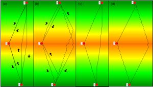
The most popular slope-dependent cost function in archaeological LCP studies probably is Tobler's hiking function (Tobler 1993). Tobler refers to data published by Imhof (1950), but Tobler's estimation of Imhof's data does not fit well. In particular, the narrow minimum of the Tobler function at a downhill gradient of 5% does not seem appropriate. Figure 6 shows that the critical slope of the Tobler cost function is in the range of 25 to 30%, both for the one-way (a and b) and the bi-directional paths (c and d). This agrees well with the results of Minetti (1995).
Kondo and Seino (2010) tried to adjust the parameters of Tobler's cost function on the basis of walking experiments on a well-preserved ancient route in Japan. The main drawback of this approach is that a narrow minimum is inherent in the cost function, moreover, only one male and one female subject were tested, and both were fairly inexperienced hikers.
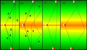
An alternative for estimating walking time is the formula published by Langmuir (2004, 40) which is implemented in GRASS GIS r.walk. This cost function is piecewise linear with three sections: ascending sections for positive and steep descending slopes, and a descending section for downhill slopes up to a negative gradient of 12° (21.25%). This cost function is discontinuous at -12°, and this does not seem intuitive. With the Langmuir cost function, the critical slope for bi-directional paths is between 20 and 25% (Figure 7c and 7d). For one-way paths the situation is somewhat different (Figure 7a and 7b). Whereas downhill LCPs include switchbacks for the 25% roof-shaped landscape, uphill paths mount the steep slope directly even for a slope of 40%. However, this is no surprise after the analysis of the simple piecewise linear cost functions above.
For estimating the slope-dependent costs of walking, Llobera and Sluckin (2007) propose using a cost function based on physiological experiments carried out in the first half of the 20th century. The main drawback of this cost function (a quartic polynomial) is that it is not a good fit with some of the values found in newer experiments by Minetti et al. (2002; Table 2). Furthermore, the minimum of this function is at a downslope gradient of 17.7%, though a minimum at a negative slope of 10% is suggested by treadmill experiments (Minetti et al. 1993). The experiments of Kondo and Seino (2010) suggest a minimum at about 7%, but this is possibly because the data of inexperienced hikers was evaluated. For this quartic polynomial, the critical slope for bi-directional and one-way paths is between 20 and 25%.
| Math. slope | Cw | Std dev. | Llobera and Sluckin | Llobera and Sluckin diff. | Minetti | Minetti diff. |
|---|---|---|---|---|---|---|
| -0.45 | 3.46 | 0.95 | 5.96 | 2.50 | 3.61 | 0.15 |
| -0.40 | 3.23 | 0.59 | 4.22 | 0.99 | 3.50 | 0.27 |
| -0.35 | 2.65 | 0.68 | 2.89 | 0.24 | 2.94 | 0.29 |
| -0.30 | 2.18 | 0.67 | 1.94 | 0.24 | 2.21 | 0.03 |
| -0.20 | 1.30 | 0.48 | 1.05 | 0.25 | 1.09 | 0.21 |
| -0.10 | 0.81 | 0.37 | 1.34 | 0.53 | 1.13 | 0.32 |
| 0.00 | 1.64 | 0.50 | 2.64 | 1.00 | 2.50 | 0.86 |
| 0.10 | 4.68 | 0.34 | 4.78 | 0.10 | 4.90 | 0.22 |
| 0.20 | 8.07 | 0.57 | 7.66 | 0.41 | 7.88 | 0.19 |
| 0.30 | 11.29 | 1.14 | 11.20 | 0.09 | 11.18 | 0.11 |
| 0.35 | 12.72 | 0.76 | 13.21 | 0.49 | 13.02 | 0.30 |
| 0.40 | 14.75 | 0.61 | 15.37 | 0.62 | 15.10 | 0.35 |
| 0.45 | 17.33 | 1.11 | 17.69 | 0.36 | 17.60 | 0.27 |
| SUM TOTAL | 7.83 | 3.56 |
In the paper by Minetti and his co-authors, a quintic polynomial is presented with better fit to the data. However, for walking on level ground, the energy expenditure estimates given by this polynomial is outside the range determined by the standard deviation of the Minetti et al. (2002) experiments. Moreover, this function is not appropriate owing to negative cost values for steep downhill slopes. When using the absolute value of this polynomial, the critical slope for descending is between 10 and 15%, whereas the critical slope for uphill movement is between 20 and 25%. The minimum of this function is at a downhill slope of 15.25%.
Owing to the drawbacks of both the quartic and the quintic polynomial, a sixth degree polynomial was constructed which fits the data found by Minetti et al. (2002):
Cost(s) = 1337.8 s6 + 278.19 s5 - 517.39 s4 - 78.199 s3 + 93.419 s2 + 19.825 s + 1.64
where s is mathematical slope and the costs are measured in terms of kilo-joule expended for each kg of the walker covering 1m. This cost function shows most of the desired properties discussed above: for both steep negative and positive slopes the costs increase, the minimum of the curve is at a downhill gradient of about 10.5%, and all the estimates are within the range given by the standard deviations. However, the critical slopes of downhill and uphill one-way paths differ widely: Whereas the critical slope of downhill walking is between 10 and 15%, for uphill movement a critical slope between 35 and 40% was found in tests with the roof-shaped landscape. For bi-directional paths, the sixth degree polynomial has a critical slope in the range of 15 and 20%, which is well below the 25% found by Minetti (1995). So the sixth degree polynomial avoids some disadvantages of the other cost functions based on physiological data, but probably only the bi-directional version is adequate for LCP calculations.