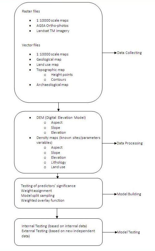
Figure 1: Steps to creating the predictive model

As shown in Figure 1, the first step in the setting up of the predictive model was to collect the cartographic dataset related to the Pisa coastal plain, both in raster and vector format. Basically it consists of 1:10K scale topographic and ortho-photographic maps, from which specific thematic layers have been derived, such as lithology and land use. Three further layers were added, obtained from a Digital Elevation Model of the study area (Figure 2): elevation, slope and aspect maps.
Figure 1: Steps to creating the predictive model

Once the cartographic dataset was implemented in a GIS database, it was necessary to identify the best strategy to fulfil the aims of the final predictive model. After analysing several case studies in which predictive modelling had been employed, we decided to use an inductive approach, which reaches the final outcome starting from an existing sample of known sites by assessing the influence exerted on this sample by different environmental variables (Wheatley and Gillings 2002).
Thus, five 'predictors' were identified and then processed by using a GIS Spatial Analyst tool. The selection of predictors was made based on the existing correlation between known sites and classes of each predictor (the higher the density value expressed by each class [surface width/no. of sites], the higher the weight assigned to it). Therefore, the variables selected as predictors were: lithology, land use, elevation, aspect and slope. In order to obtain a more reliable model, the original sample of known sites was been split into two, 'training' and 'testing', on which we set up two different predictive models that were subsequently compared and verified in their discrepancy level.
All of the predictors were then processed through a weighted overlay algorithm, obtaining the final outcome by the sum of the different weights and scores expressed by each one of them (Table 2) and finally got to the two different 'training' and 'testing' risk maps (Figure 3), both expressing three levels of probability/risk of finding new archaeology, ranging from level 1 (low risk), to level 3 (high risk).
Table 2: Weighted overlay algorithm applied to predictors
| Predictor | Variable | Value (%) | Score | Weighted value | ||
|---|---|---|---|---|---|---|
| Train | Test | Train | Test | |||
| Aspect | NW | 5 | 1 | 1 | 0.05 | 0.05 |
| SE | 2 | 1 | 0.1 | 0.05 | ||
| SW | 1 | 1 | 0.05 | 0.05 | ||
| W | 2 | 3 | 0.1 | 0.15 | ||
| E | 2 | 2 | 0.1 | 0.1 | ||
| S | 1 | 2 | 0.05 | 0.1 | ||
| NE | 3 | 3 | 0.15 | 0.15 | ||
| N | 3 | 2 | 0.15 | 0.1 | ||
| flat | 2 | 1 | 0.1 | 0.05 | ||
| Land use | Arable | 10 | 3 | 3 | 0.3 | 0.3 |
| Urban areas | 1 | 3 | 0.1 | 0.3 | ||
| Woodland | 1 | 1 | 0.1 | 0.1 | ||
| Covered area | 1 | 1 | 0.1 | 0.1 | ||
| Slope | Flat | 5 | 2 | 2 | 0.1 | 0.1 |
| 1 | 3 | 3 | 0.15 | 0.15 | ||
| 2 | 1 | 1 | 0.05 | 0.05 | ||
| 3 | 3 | 3 | 0.15 | 0.15 | ||
| Lithology | Alluvial deposits (Hol) | 60 | 1 | 1 | 0.6 | 0.6 |
| Calcarenites and sands (Ple) | 1 | 1 | 0.6 | 0.6 | ||
| Sand deposits (Hol) | 3 | 3 | 1.8 | 1.8 | ||
| Elevation (m) | 0-1 | 20 | 1 | 2 | 0.2 | 0.4 |
| 2-3 | 1 | 2 | 0.2 | 0.4 | ||
| 4-5 | 3 | 2 | 0.6 | 0.4 | ||
| 6-7 | 3 | 2 | 0.6 | 0.4 | ||
| 12-13 | 1 | 1 | 0.2 | 0.2 | ||
© Internet Archaeology/Author(s)
University of York legal statements | Terms and Conditions
| File last updated: Thu Dec 1 2011