According to Husdal (2000, 11), the first algorithms for LCP calculation were published in 1958, and 222 algorithms were known by 1979. The focus of this article is on LCP calculations that rely on costs that can be derived from one or more raster grids. Typical raster grids for LCP calculations are digital elevation models (DEM) or land cover raster maps. For raster grids, most approaches consist of a two-step process (Conolly and Lake 2006, 252; Wheatley and Gillings 2002, 157; van Leusen 2002, chapter 6, 8). The first step is to create an accumulated cost-surface (ACS) that models the accumulated cost for travelling outward from the point of origin. The second step is to identify the LCP by backtracking from the destination to the origin.
Lock and Pouncett (2010) think that 'technical accuracy' of the LCP algorithm and the geographic data are not as important as most authors think, because of the individual component in choosing the next step of a route. If this was true, many of the ideas and discussions in the present article would be obsolete. However, ancient paths often developed over a long period of time and were not formed by a single individual but are the result of the experience of many. It seems that even animals optimise their paths (Ganskopp et al. 2000), and a class of path optimisation algorithms has been inspired by experiments with ants (Dorigo 2007). Moreover, reconstruction attempts for known historical routes show that algorithms of improved technical accuracy often perform better than those with significant deficiencies (e.g. Herzog 2009b).
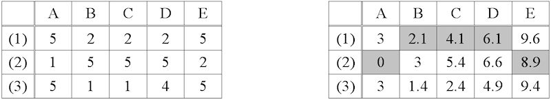
The ACS is centred on the origin, which is assigned a cost of zero. Each cell of this ACS contains the costs of reaching this cell from the origin (e.g. Bell and Lock 2000). The process of generating an ACS is best illustrated for a cost model where each raster cell is associated with the cost for crossing the cell, and the costs are independent of the direction of the traversal. The term isotropic cost grid is often used in this context (Wheatley and Gillings 2002, 151; Conolly and Lake 2006, 215; Husdal 2000, 13–14; Worboys and Duckham 2004, 145–6). Successively, the accumulated costs for reaching all cells are calculated by spreading from the starting point (e.g. Smith et al. 2007, 142-3; Yu et al. 2003).
The spreading process is implemented stepwise, and each step can be compared to a move on a chessboard. At the starting point the accumulated cost is 0. Now consider the four nearest neighbouring cells of the starting point (which can be reached by the rook's (castle) move on a chess board). The accumulated cost for a move of this sort is the average of the costs assigned to the starting point and the neighbour considered. The cost of a diagonal move is the average as well, but multiplied by 1.4142 (square root of 2) to account for the longer distance between the cell centres (Figure 1). For simplicity, the ACS in Figure 1 relies on moves in eight directions (Queen's moves on a chess board); however, taking more directions into account improves the outcome (see below).
Most LCP implementations in GIS software are based on the algorithm published by Dijkstra in 1959 (Cormen et al. 2001, 595–9; Worboys and Duckham 2004, 215–16). However, this algorithm is designed for weighted graphs with positive weights. So the first step in the LCP algorithm is to convert the raster data to a weighted graph. A weighted graph is a network of nodes (i.e. locations) and weighted links (i.e. connections between the nodes, where the weights are the costs for travelling along the link). If the centres of the grid cells are considered as graph nodes and the moves to the neighbouring cells are the links, with the weight calculated as explained above, then the vector algorithm can be applied to raster data and the optimal cost path is found (Collischonn and Pilar 2000; Husdal 2000, 13; Llobera 2000; Yu et al. 2003).
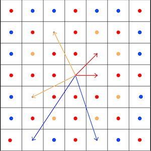
The raster to graph conversion is illustrated in Figure 2. This conversion introduces elongation errors (Huber and Church 1985) i.e. although the true optimal path between any two points on a surface with uniform friction is a straight line, the LCP calculated on the basis of the links forming the graph is often longer and includes bends, because it consists of successive moves to neighbours. For this reason, most LCPs connecting any two locations are longer than the true optimal path. Within a 7 x 7 neighbourhood, the elongation error is avoided when the raster to graph conversion includes Queen's, Knight's as well as A- and B-moves. A- and B-moves are comparable to Knight's moves, but whereas Knight's moves consist of 2-1 steps, A-moves are 3-1 steps, and B-moves are defined by 3-2-steps. Most LCP software currently available supports only Queen's moves; GRASS GIS includes an option for Knight's moves.
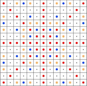
But even if A- and B-moves are implemented, the cells marked by grey dots in Figure 3 still cannot be reached from the origin by a straight line connection. Huber and Church (1985) list the worst case elongation errors depending on the neighbourhood size considered. The worst error is about 8% for paths including only Queen's moves, a reduction to 2.8 or 1.4% can be achieved by supporting Knight's moves or A- and B-moves respectively. It is important to minimise the elongation error, when the aim is to construct a cost-efficient connection between two locations.
However, most archaeological LCP studies focus on reconstructing optimal routes, and therefore, the worst case distance between the optimal route and the LCP is a more important performance indicator than the elongation error. This worst case distance is 20% of the path length if the LCP consists of Queen's moves only; including Knight's moves introduces a reduction to 11%; additional A- and B-moves cut down the worst case error to 4.6% (Herzog 2013b).
For this reason, only LCP software supporting Knight's moves or even A- and B-moves is appropriate for LCP calculations aiming to reconstruct routes. Some experiments with standard LCP software showed that this issue is not only relevant in theory, but also occurs in practice (e.g. Herzog 2013b; Herzog and Posluschny 2011). However, computation time increases considerably when Knight's moves and A- as well as B-moves are included in the LCP calculations.
Furthermore, Knight's, A- or B-moves may skip over small local barriers unnoticed. Even diagonal moves can cross high-cost barriers consisting of corner-connected cells (van Leusen 2002, chapter 16, 14–16, fig. 13) without paying the appropriate costs. Van Leusen used a neighbourhood of eight cells, and in this case, increasing the breadth of the barrier to two cells addresses the problem properly. When adjusting this workaround for A- and B-moves, barriers consisting of four consecutive cells are required. In fact, grid resolution is increased by allowing simple long moves (Rowe and Ross 1990).
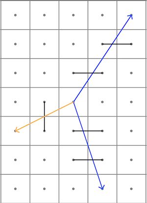
Subdividing the Knight's move into two submoves and A- as well as B-moves into three steps ensures that appropriate costs are paid when traversing barriers (Figure 4; Herzog 2013b). The costs of reaching the intermediate stops are calculated by taking the distances to each of the two neighbouring cells into account. This is only a very crude estimate for the costs of reaching the intermediate points; however, any more refined approach increases the computational load. In fact, the method proposed is equivalent to inverse distance weighting interpolation (e.g. Smith et al. 2007, 294–5) with setting the search radius to the grid resolution, so that the interpolation result depends only on the values of two neighbouring cells.
The arguments above assume that the grid cells are – nearly – squares in reality. So an adequate projection of the geographic data is required. Longitude/latitude data such as ASTER DEM delivered in WGS84 projection is only appropriate for LCP calculations if projected to an adequate coordinate system, for instance an equal area projection as recommended by Nelson (2000).
For each cell reached by the spreading process, Dijkstra's algorithm stores the back-link to its predecessor. So after the spreading procedure reached the target, the LCP is constructed by joining the back-links from the target to the point of origin. Unfortunately, some GIS packages do not implement Dijkstra's algorithm in all parts: First, Dijkstra's method is applied to generate the ACS, and thus the cost of the optimal path is known. Afterwards, the route of steepest cost reduction is located by a drainage algorithm which does not necessarily track the back-links (Smith et al. 2007, 146).
Such drainage or steepest descent algorithms can be implemented easily and do not require additional memory for a back-link grid. However, Smith et al. (2007, 146) note that paths generated by steepest descent may become trapped in localised plateaux or pits, and they list several other disadvantages of this method. Bellavia (2002) describes quite a complicated drainage procedure that involves filling the pits of the cost surface.
When looking for examples illustrating the fact that steepest descent does not always identify the LCP, initially, the only relevant reference found was the thesis by Husdal (2000, 18–19), summarising work of McIlhagga – but unfortunately, this example is mathematically not correct. Later a correct example was found in Smith et al. (2007, 146) and another one is presented in Figure 1: the steepest descent from cell E(2) is to cell D(3), as the difference of the accumulated costs is greater than that to D(1) and the distance from E(2) to D(1) is the same as that from E(2) to D(3). But the cost for moving from D(3) to E(2) is 4.2, resulting in an accumulated cost of 9.1 in E(2) which exceeds 8.9, i.e. the sum of 6.1 and the cost of moving from D(1) to E(2).
Currently, ESRI's costdistance procedure (ArcGIS 9.2) implements Dijkstra's algorithm including back-links. The GRASS GIS procedures r.cost and r.walk in the stable version 6.4 were improved a few years ago so that a subsequent call to r.drain is able to track back-links. The grid for storing the back-links is called movement direction surface in GRASS (checked on 11 April 2014).
In 1983 Tomlin suggested a less effective iterative method for ACS calculation (Tomlin in Husdal 2000, 14; Conolly and Lake 2006, 221–3) that is simpler to implement than Dijkstra's algorithm because it does not require a priority queue. It seems that Tomlin's and Dijkstra's ACS results are identical.
Rowe and Ross (1990) note that one of the disadvantages of raster based LCP calculations is the fact that much computation time is wasted because the search for the goal is mostly blind. The A* search algorithm (Worboys and Duckham 2004, 216–17; Husdal 2000, 12), which belongs to the class of informed search algorithms, is a modification of Dijkstra's algorithm that reduces the computational load in most situations considerably by taking the distance to the goal into account.
My LCP algorithm implementation first calculates the costs of the direct path and uses this cost value as a threshold on when to give up: whenever a cell's neighbours are to be tested, the program evaluates if this cell could possibly be part of the LCP. The sum of the accumulated costs for reaching the cell and the crow-fly-distance to the target point multiplied by the minimum cost of the currently selected cost function are calculated, and if this value exceeds the cost of the direct path, this cell is no longer considered a candidate for a location on the LCP. In addition, whenever the target point is reached with a lower total cost than that of the direct path, the threshold value is updated accordingly. This method works only if all costs are positive.