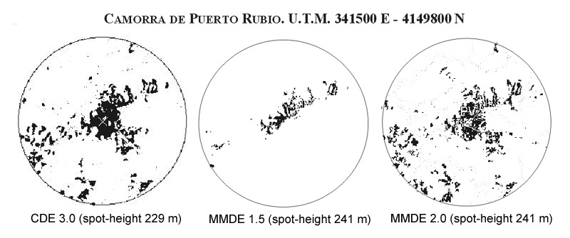
That the inherent inaccuracy of DEM (Digital Elevation Model) leads to divergent viewsheds for a given point has been largely acknowledged and graphically illustrated (e.g. Mandry and Rakos 1996; Zamora 2006) (Figure 7).
Figure 7: Viewsheds from the same viewer point (Camorra de Puerto Rubio U.T.M. 341500 E - 4149800 N) using three different DEMs (derived from the Spanish army digital maps CDE 3.0, MMDE 1.5 and MMDE 2.0). The visible area is shown in black. The spot-height plotted on every digital map for the quoted coordinates is given in brackets. It is clear that the viewshed from the same viewer point differs significantly depending on the DEM (Zamora 2006, 45, fig. 2).
The geographer Fisher recognised this problem and suggested a method to accommodate such errors, the probable viewshed, where the visibility of every cell is indicated not through a binary system but in terms of probability of being seen (Fisher 1991, 1992, 1993 and 1994; Nackaerts et al. 1999; Wheatley and Gillings 2000, 10-11 and 2002, 209-10). However, archaeological publications making use of his technique are rare, a remarkable exception being a project that implements probable viewsheds to investigate the visual relationships between different elements of the defence system around the ancient city of Salagassos (Turkey) (Nackaerts and Govers 1997; Loots et al. 1999 and Nackaerts et al. 1999) [note 3].
3.2.2 General criteria and procedure
Essentially, the technique proposed is that of Fisher (1992, 345).
a) Obtaining a number of simulated DEMs containing error
The DEM error
Simulated DEMs can be obtained by means of Monte Carlo techniques where random fields of error are generated and subsequently added to the original DEM.
Monte Carlo simulations do not aim to achieve 'the true DEM', just DEMs that contain error of the same nature as is believed to exist in the original DEM (Eastman 2006, 159). That is to say, the simulated DEMs aim to represent how X metres of error could have affected the structure of the original DEM. Because of this, field errors need to be generated taking into account the RMSE (root-mean-squared error) of the original DEM. As detailed in the discussion of the data sources, the published RMSE of the DEM acquired for this study is 1.39m for areas of non-complex topography. For this first implementation of probable viewshed it has been assumed that the published error is equally distributed over the study area.
It can be noted that the quoted 1.39m error can be considered a low value. For example, the DEM used by Fisher (1991 and 1992) had a published error of 7m, whereas the error for the DEM employed in the archaeological study of Salagassos was estimated as 10m (Nackaerts and Govers 1997, 4).
The number of simulations
A total of 20 simulated DEMs were generated following the model established by Fisher (1991 and 1992). It was deemed unnecessary to increase the number of simulations since the resultant viewsheds were very similar, presumably a result of the low DEM error.
The algorithm
Fisher (1991, 1322) described and implemented two algorithms in order to generate fields of error and add them to the original DEM. The first does not take into account spatial autocorrelation whereas the second measures autocorrelation using Moran's I index.
In its most general sense, spatial autocorrelation is concerned with the degree to which features from a given location are similar to other features located nearby (Goodchild 1986, 3). A given DEM should have cell values mostly similar to their neighbours i.e. autocorrelated. For example, if the elevation at point X is 250m, the elevation at point Y, 10m from X, can be expected to be in the range 240 to 260m. A remarkable difference between X and Y would indicate, for example, the existence of a cliff (O'Sullivan and Unwin 2003, 28). In contrast, the values of a field of error should not be dependent on each other, since it is meant to introduce scattered random errors in the original DEM. In other words, a field of error should have no autocorrelation; otherwise clustered error could form occasional bulges and distort areas of the DEM (O'Sullivan and Unwin 2003, 187; Englund 1992, 3; van Niel and Laffan 2003, 52).
While ignoring autocorrelation may be deemed acceptable (e.g. Nackaerts and Govers 1997), I would argue that testing of the autocorrelation of error fields is a crucial stage in the process. Therefore, this research implements the second algorithm described by Fisher; however, autocorrelation is assessed using a different procedure.
Monte Carlo techniques for generating random DEMs were carried out within Idrisi 32. Fields of error were generated through the module RANDOM (Eastman 2006, 159; Rossiter 1994). Once a given field of error had been created, and before adding it to the original DEM, its degree of autocorrelation was measured by means of the Idrisi's AUTOCORR module.
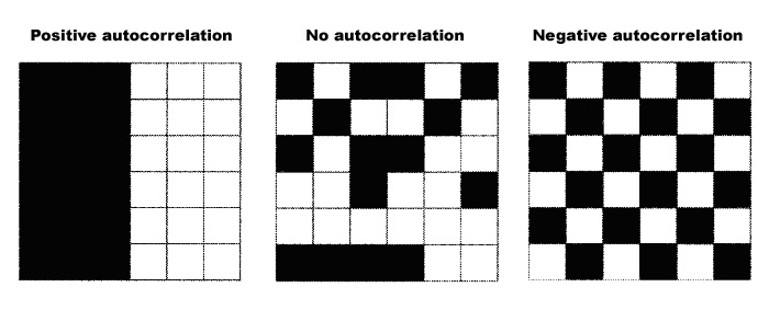
AUTOCORR calculates the first lag autocorrelation coefficient using Moran's I index. First lag autocorrelation examines the spatial dependence for the adjacent neighbours of a cell. It can be tested either by using Rook's case, which bases autocorrelation on a pixel's four immediate neighbours, or King's case, which measures autocorrelation for the surrounding eight neighbours of a cell (Eastman 1997, 5, 7). For this study, King's case was chosen. Moran's I index indicates the degree of autocorrelation in a range from -1 to 1 (Figure 8). Moran's I index is positive when nearby values tend to be similar (i.e. autocorrelated), approximately zero when values are arranged randomly and independently in space (no or 0 autocorrelation), and negative when they are more dissimilar than expected (negative autocorrelation) (Eastman 1997, 18, 67; Goodchild 1986, 16; O'Sullivan and Unwin 2003, 187). In practice, the module AUTOCORR indicates that the expected value if there is no autocorrelation is -0.0000.
In the current study a threshold value of the Moran's I index from -0.0000 to -0.0010 was established. When the autocorrelation of a given error field fell within that threshold, the field was added to the original DEM using OVERLAY. If the autocorrelation was outside the threshold, the error field was rejected and subsequent error fields were generated until one with the predetermined level of autocorrelation was obtained.
b) Calculating a viewshed for every DEM
Once the simulated DEMs had been created a viewshed for every simulated DEM (as well as for the original DEM) was generated. As explained in section 3.1.2, the viewshed for each hillfort included five viewer positions.
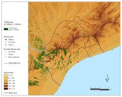
Additionally, one probable viewshed from a single viewer position was performed for the hillfort known as Puig Castellar (Figure 9) with the aim of better illustrating the procedure and discussing the results.
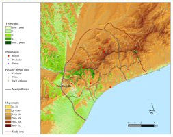
Figure 9 (left): Probable viewshed from 1 viewer point (from Puig Castellar hillfort). Figure 10 (right): Probable viewshed from 5 viewer points (from Puig Castellar hillfort)
c) Summing the resultant viewsheds
The viewsheds generated for each simulated DEM and the original DEM were added together to yield a cumulative viewshed that shows the likelihood of any location being seen from the hillfort.
When a single viewer point is used (Figure 9), the probable viewshed reflects how many DEMs a given cell can be seen in. Obviously, areas that are seen in a greater number of DEMs have a greater probability of actually having been seen than those visible from a low number of DEMs, which might be due to DEM inaccuracies.
When multiple viewer points are taken into account (Figure 10), the probable viewshed shows how many times, including viewer points and DEMs, a given cell is seen. The values include both viewer points and DEMs. For example, a value of 21 could indicate that an area is seen once from 21 DEMs or from more than one viewer point in less than 21 DEMs. Cells with the highest value, 105, are seen from all DEMs and all viewer points (21 DEMs x 5 viewer points = 105).
d) Dividing the probable viewshed by the number of DEMS
Additionally, as pointed out by Nackaerts et al. (1999, 63), the sum of all the values can be divided by the number of DEMs. This results in a viewshed that shows only those cells that are visible in the entire set of DEMs employed (i.e. 21). When a single viewer point is used (Figure 11), the visible area
contains a value of 1 (hence, this area is coincident with the value 21 of Figure 9). When multiple viewer points are considered (Figure 12), the visible area has values indicating from how many viewer points a cell is seen. The latter viewshed, deemed the most likely to have actually been seen, has been selected as a basis for the next stage of the analysis: Higuchi and cumulative viewsheds. It will be referred to as the most probable viewshed [note 4]. (See the most probable viewshed of each hillfort in Figures 18, 22, 26, 30, 34, 38, 42 and 46).
Figure 11 (left): Probable viewshed from 1 viewer point: selection of the area seen from all the DEMs (from Puig Castellar hillfort). Figure 12 (right): Most probable viewshed from 5 viewer points (from Puig Castellar hillfort)
3.2.3 Discussion
If the probable viewsheds from one and multiple viewer points are compared with their respective viewsheds based on the original DEM a number of points become clear.
First of all, it can be noted that the probable viewshed from one viewer point (Figure 9) and the binary viewshed from the same point (Figure 5: top), are not essentially divergent. In terms of visible area the main difference concerns a zone south-east of the viewer point, i.e. Puig Castellar. While it would not be visible according to the binary viewshed, the probable viewshed indicates the possibility of visibility. Moreover, from the probable viewshed it may be estimated that some small areas of the binary viewshed should be considered with caution, since they are only seen in 1-2 DEMs and hence could be due to error.
The overall similarity between both viewsheds can undoubtedly be attributed to the low error quoted on the ICC DEM, and the decision to ignore the caveat concerning areas of changeable topography and apply the quoted error range to the DEM as a whole.
Thus, given a small DEM error, it could be argued that probable viewsheds are not necessary. However, differences are still evident. For example, the divergent visible area south-east of Puig Castellar questions the visual relationship between the hillfort and a group of possible Iberian sites (compareFigure 5 top, with Figure 9 and Figure 10).
Secondly, Figures 5 (centre) and Figure 10 show that there is no significant change between the ordinary and probable viewsheds when five viewer points are taken into account. This is further illustrated by the relevant viewsheds of every hillfort (Figures 16-17; 20-21; 24-25; 28-29; 32-33; 36-37; 40-41, and 44-45). Essentially, the probable viewshed indicates clearly that the edges of the viewshed should be considered less visible.
Finally, it is worth pointing out that the above-mentioned area south-east of Puig Castellar not visible in the binary viewshed (Figure 5: top) but with likelihood of visibility in the probable viewshed from one viewer point (Figure 9), appears as a visible area when performing the analyses from five viewer points (compareFigure 5: centre and Figure 12). Hence, the results of the probable viewshed would seem corroborated. Furthermore, viewsheds from multiple points would seem a simple technique with the potential to reduce errors and lead to more accurate results.