PREVIOUS   NEXT   CONTENTS   SUMMARY   ISSUE   HOME 

List of Figures

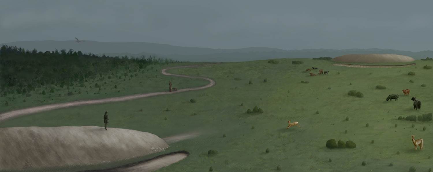
Summary page image: The Winterbourne Stoke landscape. A reconstruction by Eleanor Winter © Historic England

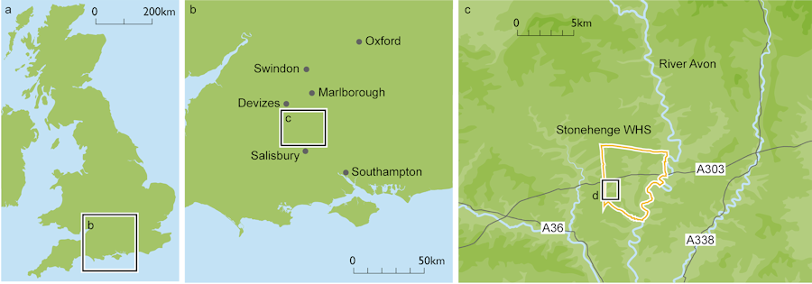
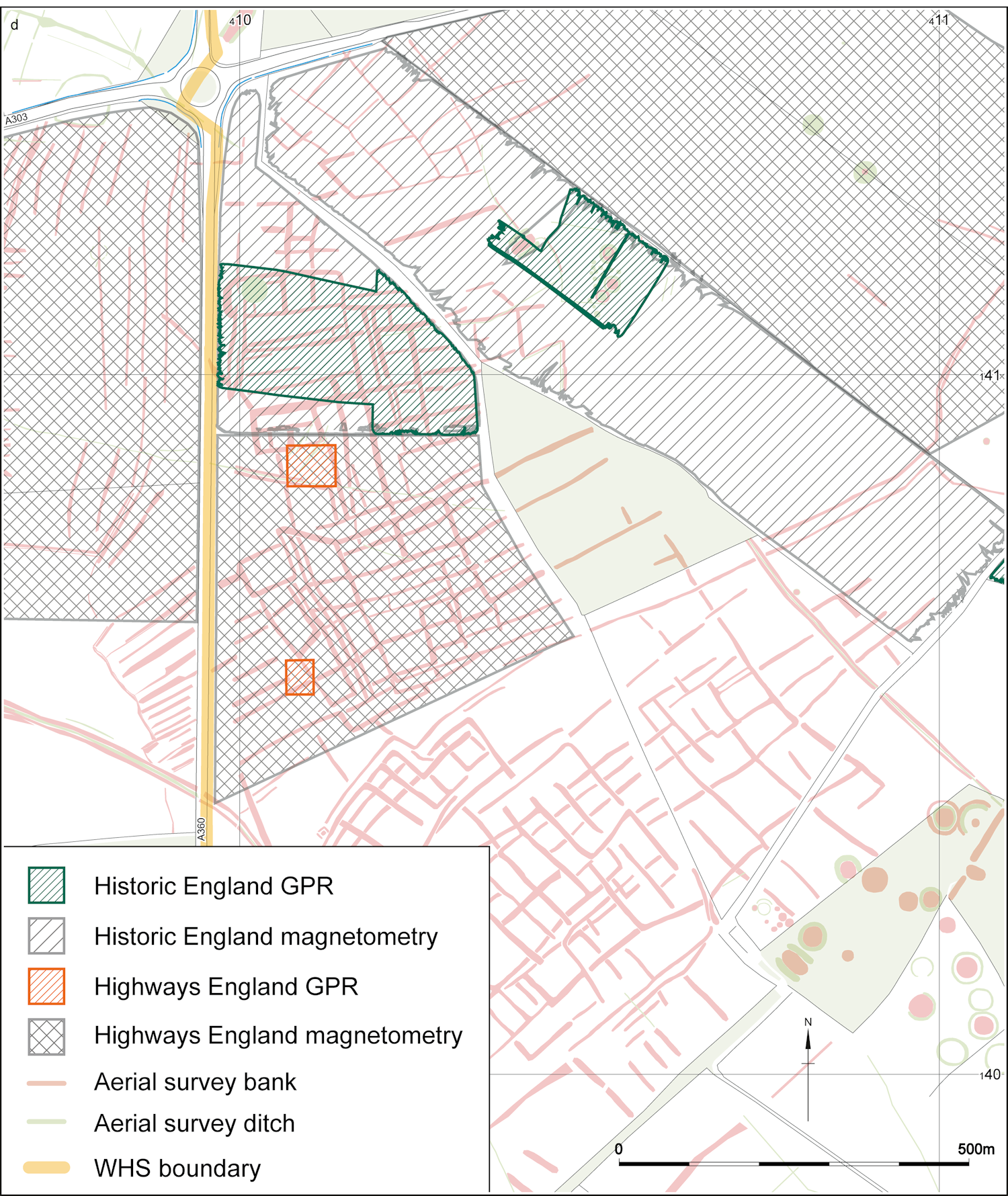
Figure 1a–c: Site location maps, Figure 1d showing aerial photographic results and areas of Historic England and Wessex Archaeology geophysical surveys. Contains data © Wessex Archaeology, reproduced with permission

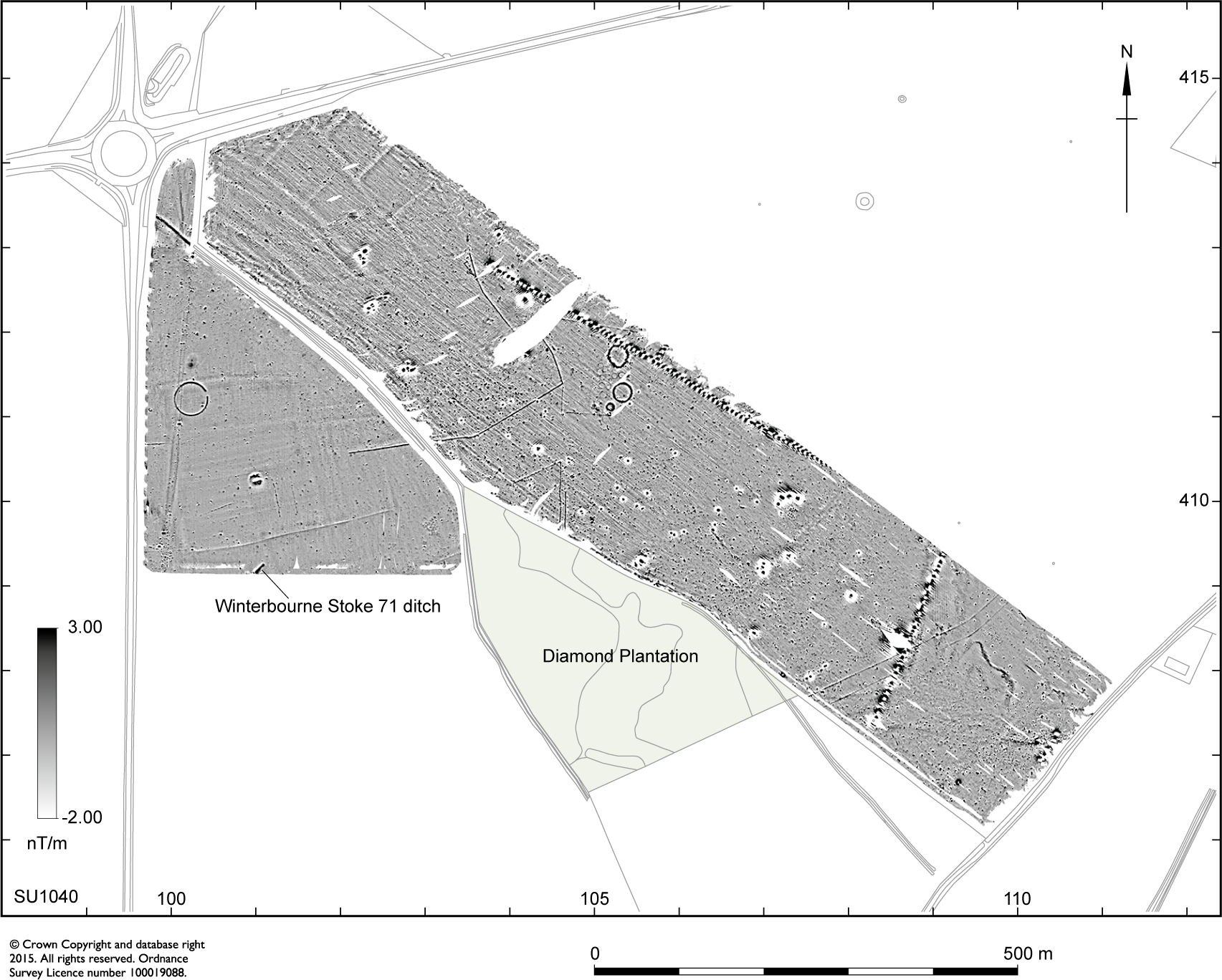
Figure 2: Historic England magnetometer survey results. Geophysical survey data provided by N. Linford (see Linford et al. 2015)

Figure 3: Wessex Archaeology magnetometer survey results. Contains data © Wessex Archaeology, reproduced with permission

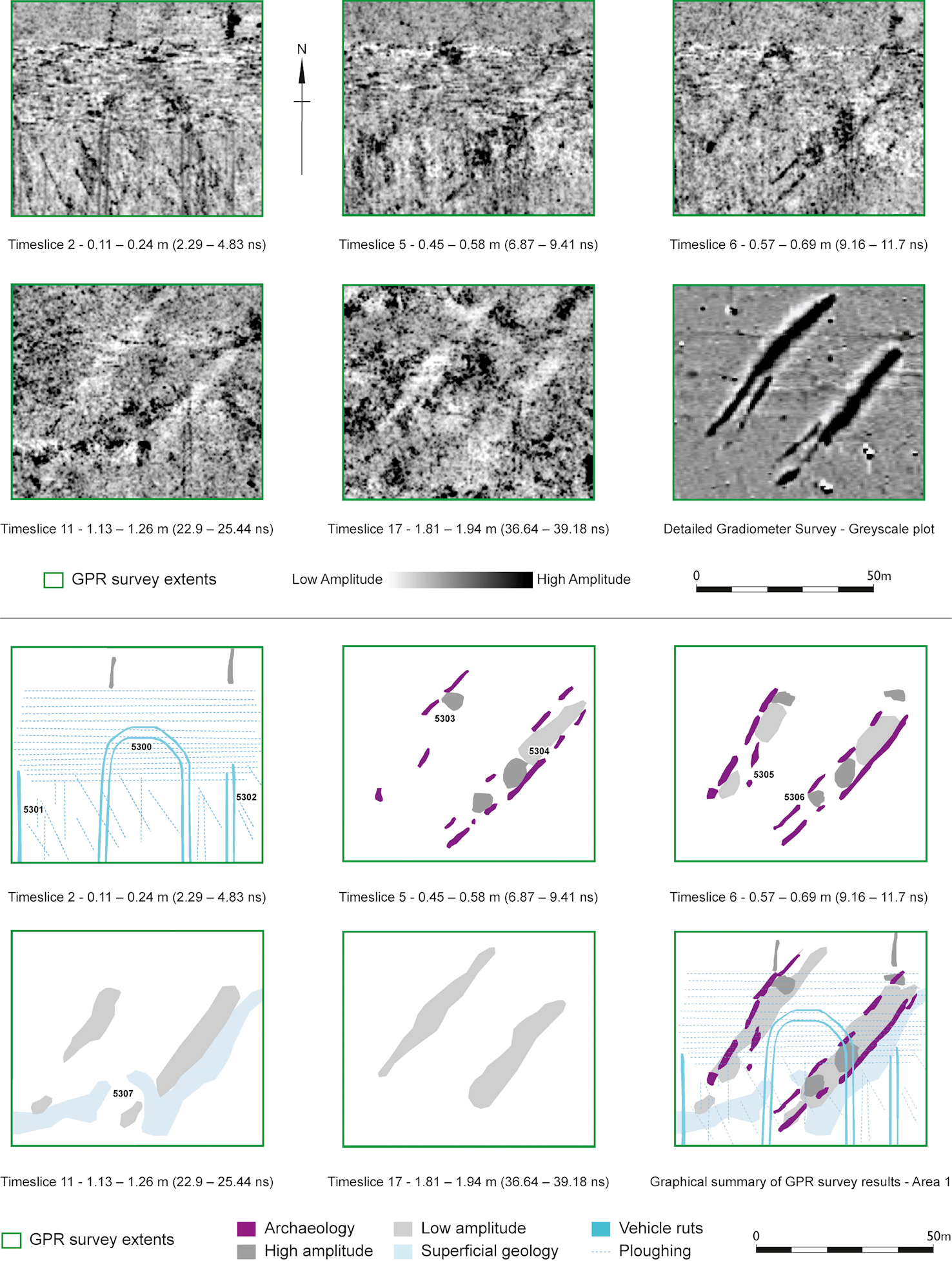
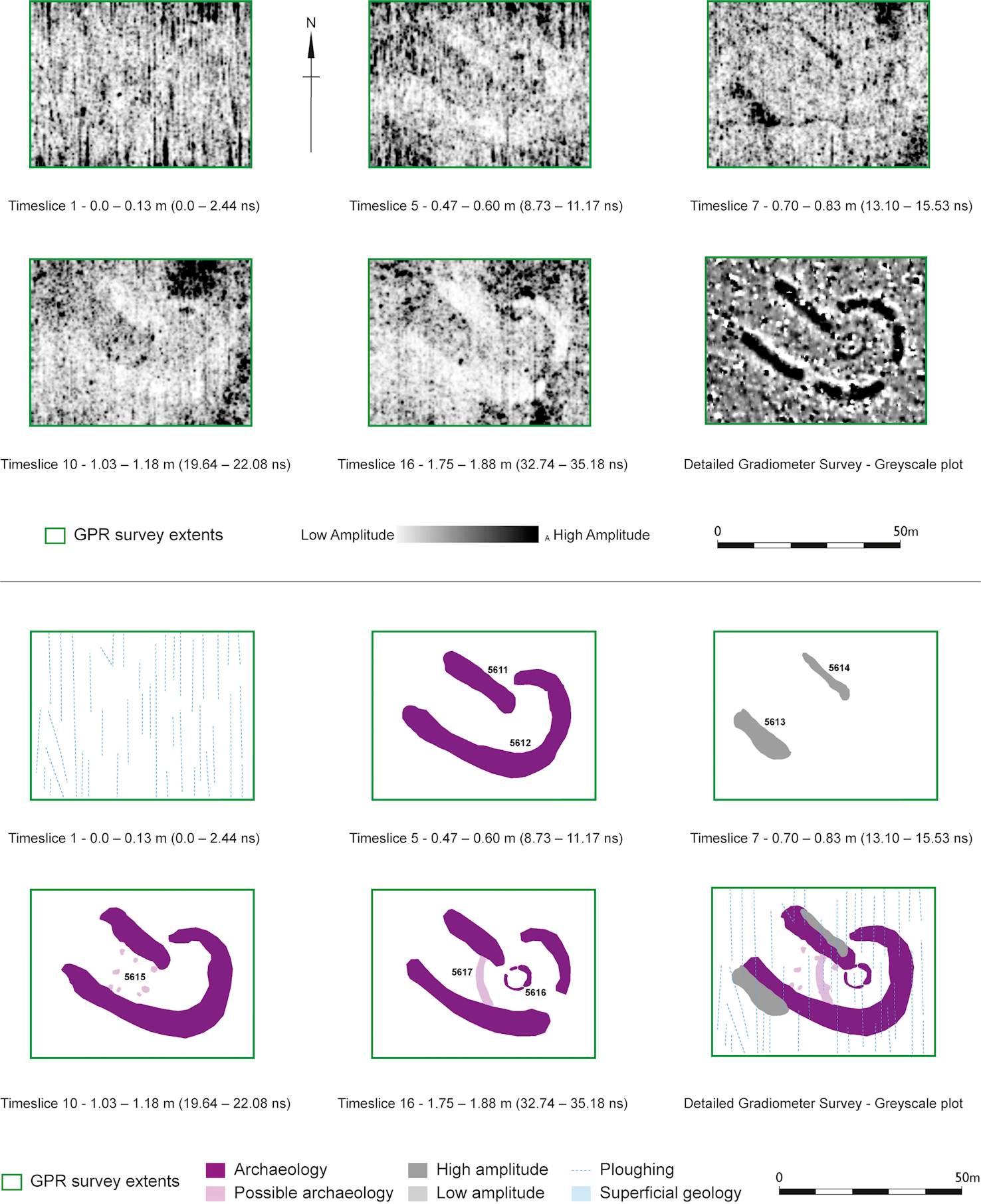
Figure 4: Wessex Archaeology GPR results (WS71). Contains data © Wessex Archaeology, reproduced with permission

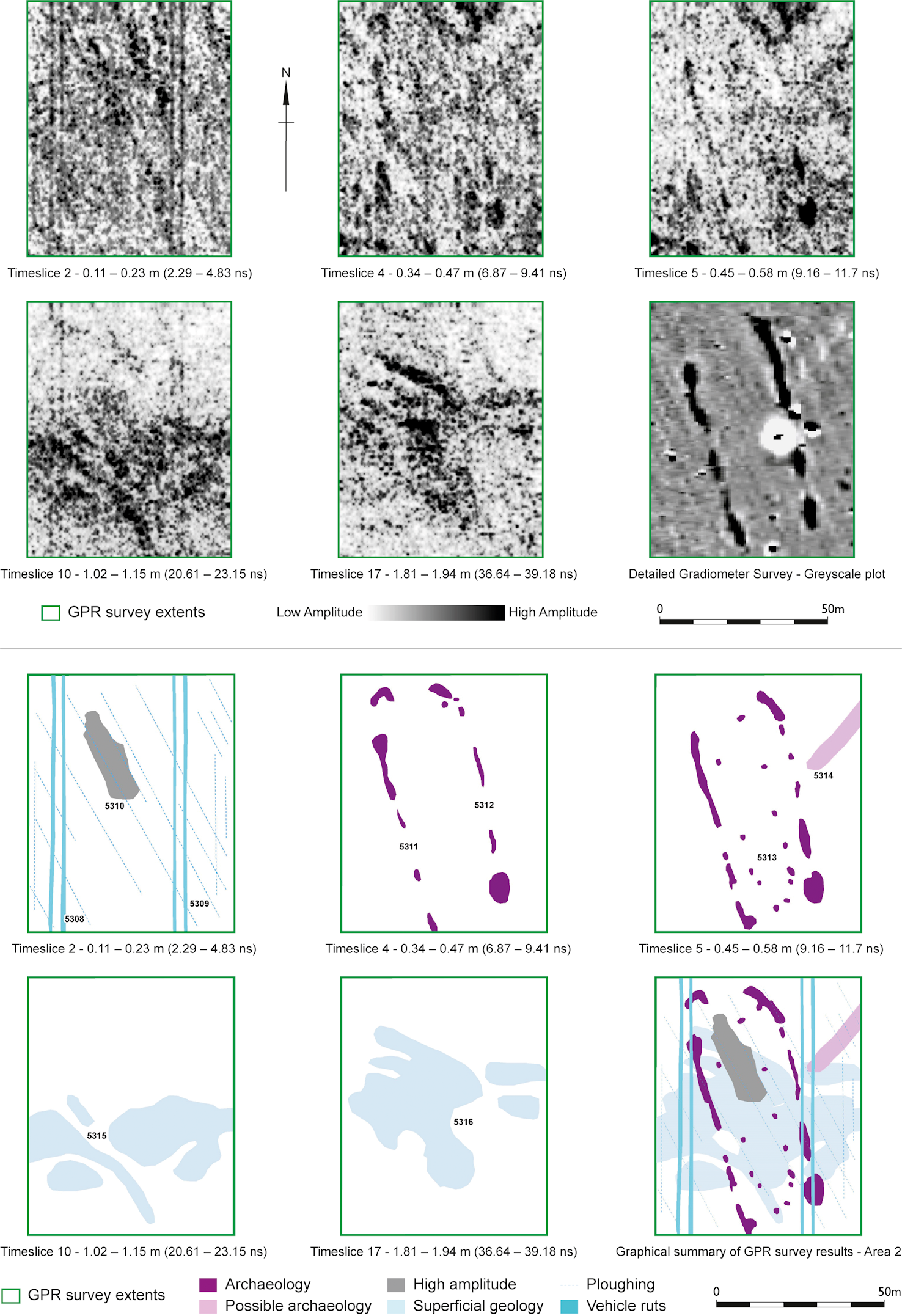
Figure 5: Wessex Archaeology GPR results (Winterbourne Stoke 86 (WS86) / HOUID 1611042). Contains data © Wessex Archaeology, reproduced with permission

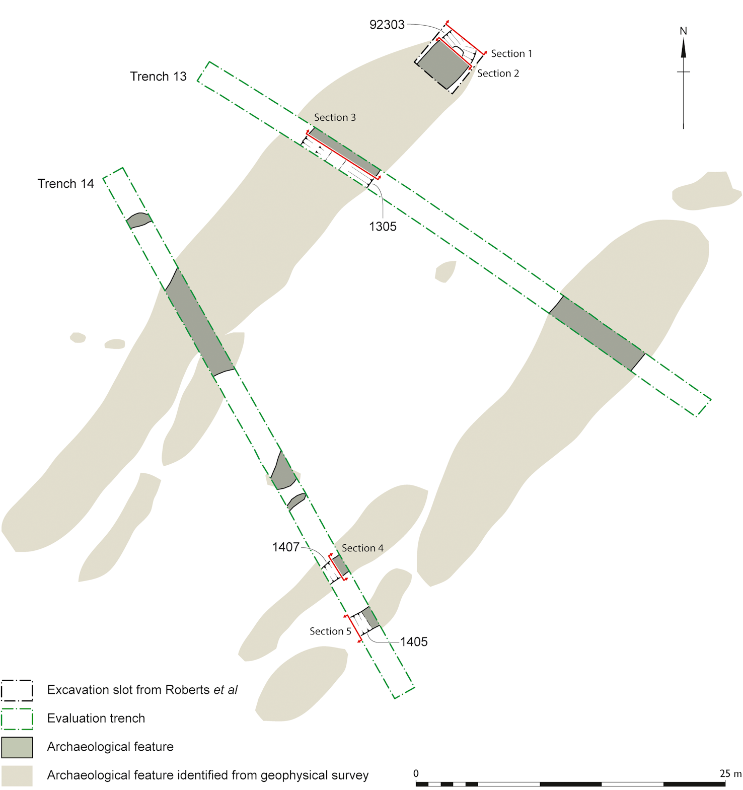
Figure 6: Plan of Historic England and Wessex Archaeology excavations of WS71. Contains data © Wessex Archaeology, reproduced with permission

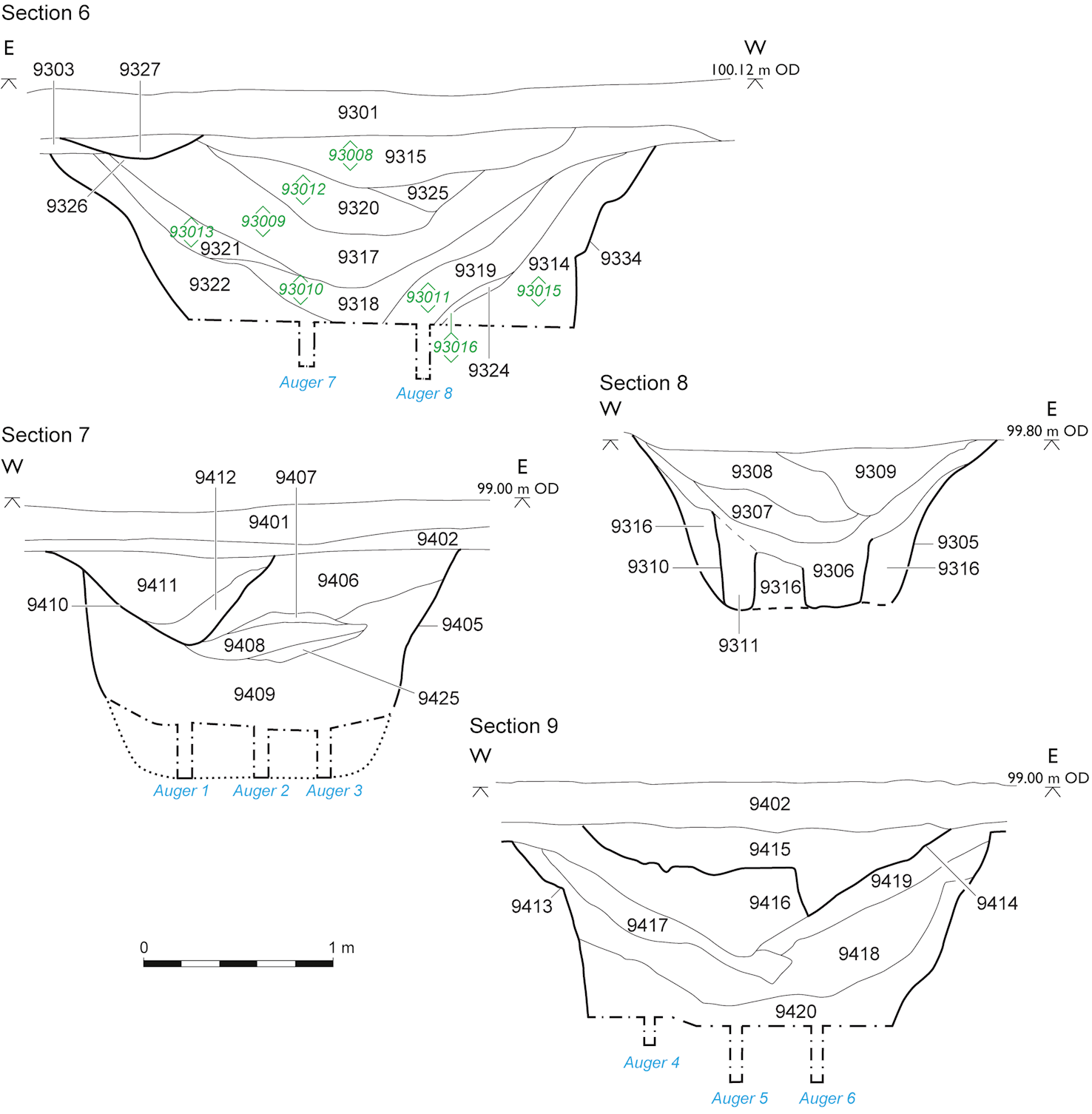
Figure 7: Sections from Historic England excavation and Wessex Archaeology excavations. Contains data © Wessex Archaeology, reproduced with permission

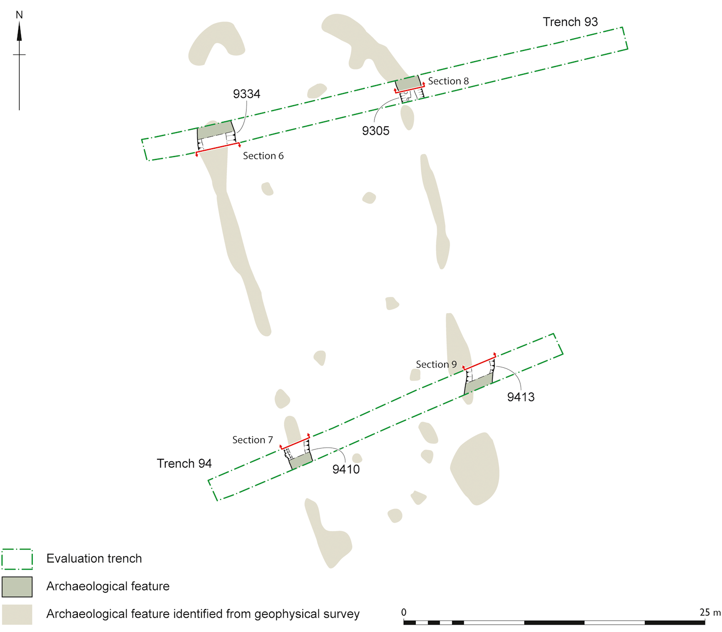
Figure 8a: Plans and Figure 8b sections of Wessex Archaeology excavations on Winterbourne Stoke 86. Contains data © Wessex Archaeology, reproduced with permission

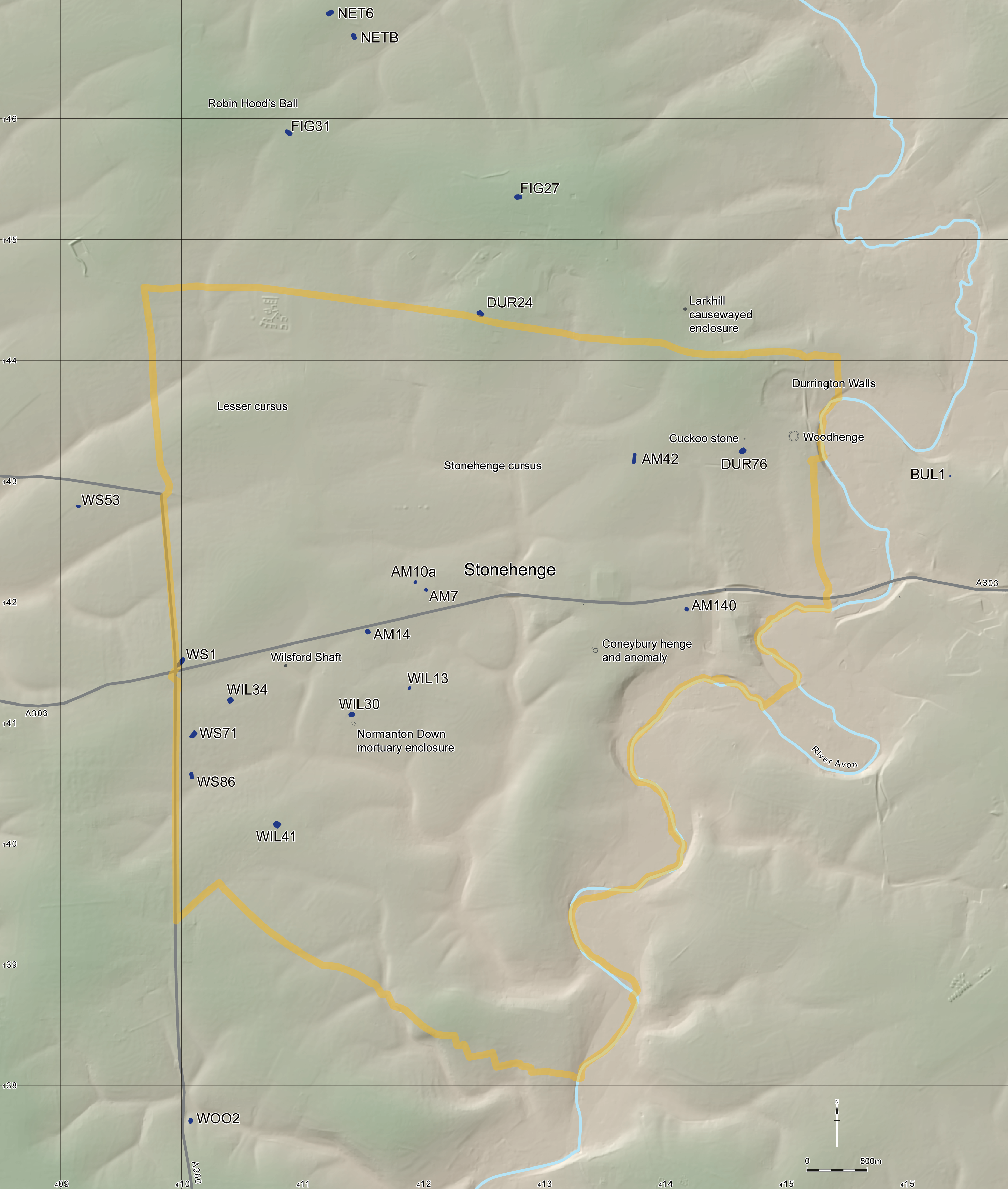
Figure 9: Distribution map of long barrows in the SWHS and environs. (Zoomable version / Clickable version)

Figure 10: Comparative simplified plans of long barrows in SWHS and environs. Green represents mounds, grey represents ditches. Based on earthwork survey and geophysical data from various sources; see individual long barrow pages via Figure 9 for information on each barrow, and sources for detailed plans

Figure 11: Wessex Archaeology GPR survey of AM140. Contains data © Wessex Archaeology, reproduced with permission

Figure 12: Dimensions of long barrows in the Stonehenge WHS and environs. All measurements are from the most recent archaeological surveys available, but as these include aerial, geophysical and analytical earthwork surveys of monuments that have suffered a wide spectrum of use, degradation and adaptation over around 5500 years, these dimensions are at best indicative of the original size of the monument. Where there is a difference in measurements taken by different methods, precedence has been given in the following order: excavation, analytical earthwork survey, geophysical survey, aerial survey. Width is defined as the maximum dimension of the area between the inner edges of the side ditches, or across the short axis of the mound if side ditches are not present. Length is defined as the long axis of the mound, or the maximum dimension of the area enclosed by ditches on the long axis of the barrow, if ditches encompass either/both ends of the mound

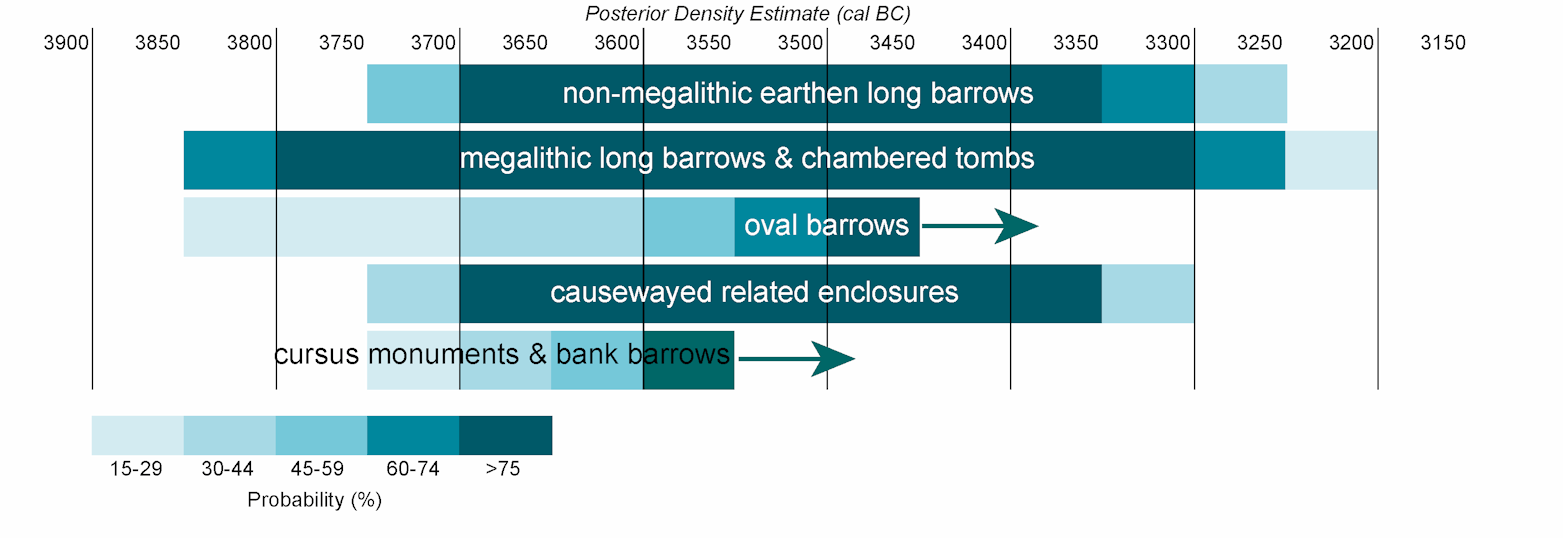
Figure 13: Schematic diagram showing the periods of use of dated monuments in south-central England of the 4th millennium cal BC. Given the difficulties in estimating when linear monuments went out of use an arrow has been used to denote when they would probably have still remained a visible feature in the landscape

Figure 14: Alignments and lengths of long barrows in the SWHS and environs

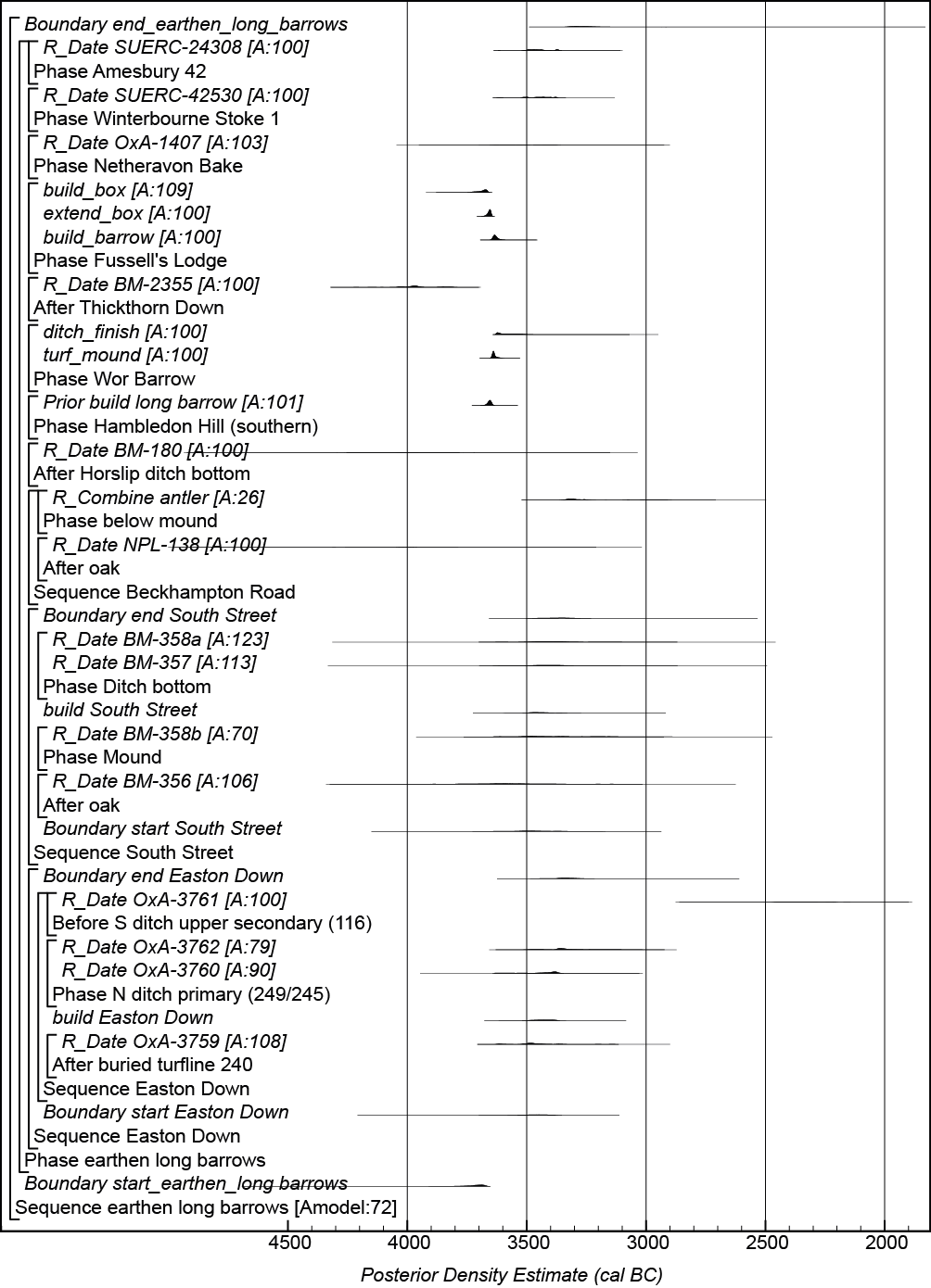
Figure 15: Probability distributions of dates from earthen long barrows from southern Britain. Each distribution represents the relative probability that an event occurred at a particular time. The distributions for the start and end of the use of individual sites have been taken from the site models described in detail in Whittle et al. (2011; figs 4.7–4.13 (Hambledon Hill)), Allen et al. (2016, fig. 12a (Wor Barrow)), and Wysocki et al. (2007b, fig. 10 (Fussell's Lodge)), and are shown in outline recalculated as necessary using IntCal13 (Reimer et al. 2013). Other distributions are based on the chronological model defined here, and shown in black. For example, the distribution 'start_earthen_long_barrows' is the estimated date when the first earthen long barrow was constructed in this area. The large square brackets down the left-hand side along with the OxCal keywords define the overall model exactly

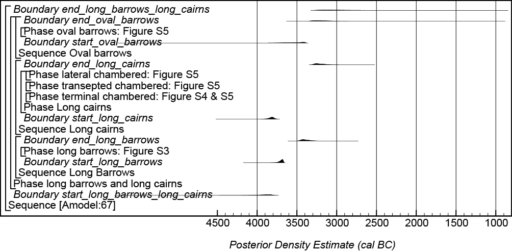
Figure 16: Probability distributions of dates from chambered long barrows, cairns, and oval barrows. The format is identical to that of Figure 15. The component sections of the model are shown in Figures 17, 18, 19. The large square brackets down the left-hand side along with the OxCal keywords define the overall model exactly

Figure 17: Probability distributions of dates for long barrows. The format is identical to that for Figure 15. Distributions have been taken from the site models described in detail in Whittle et al. (2011, figs 4.7–4.13 (Hambledon Hill)), Wysocki et al. (2007b, fig. 10 (Fussell's Lodge)); Bayliss et al. (2007, fig. 6 (West Kennet)), and Whittle et al. (2007, fig. 4 (Wayland's Smithy I)). The overall structure of this model is shown in Figure 16, and its other components in Figures 18 and 19

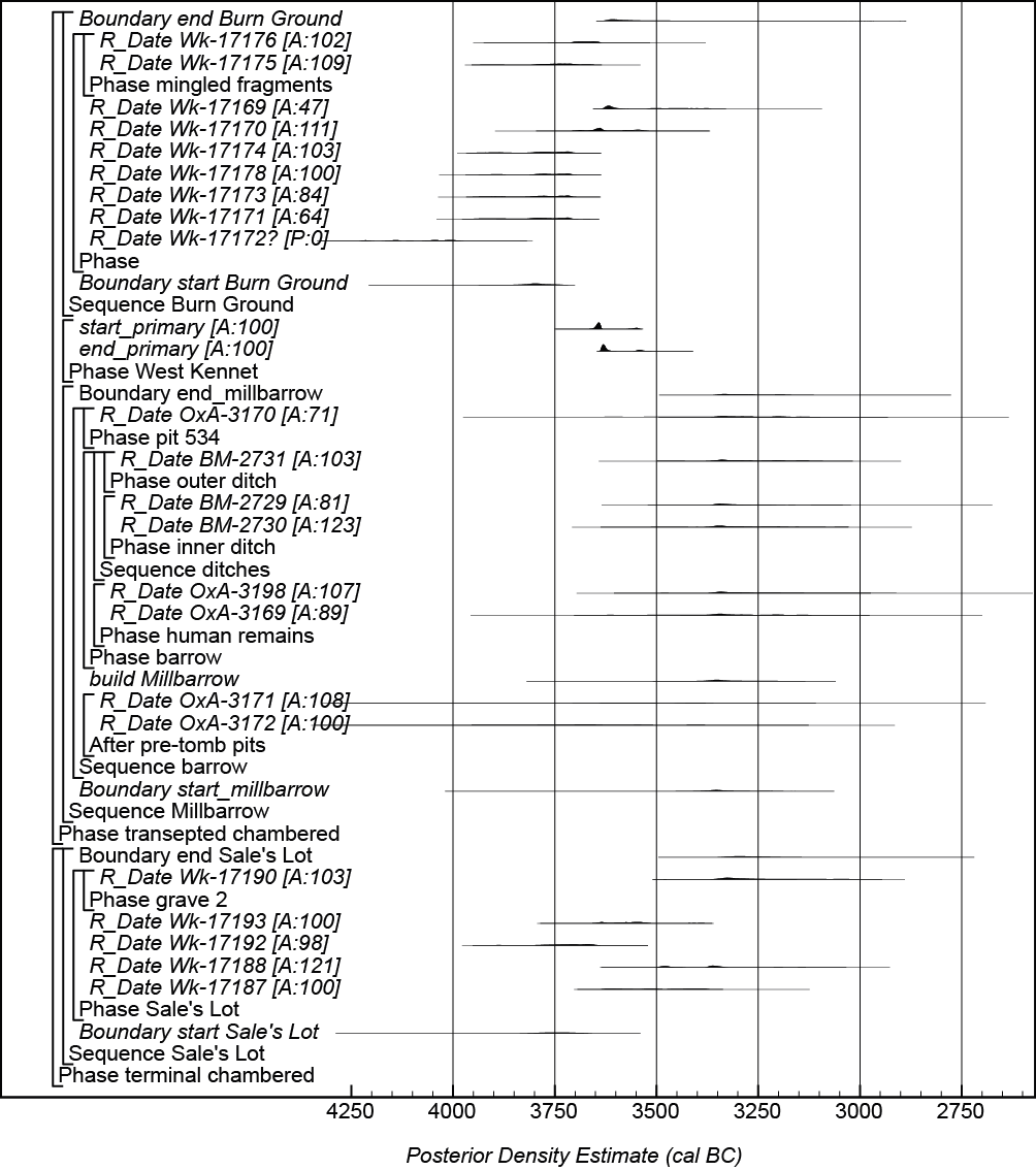
Figure 18: Probability distributions of dates for chambered tombs. The format is identical to that for Figure 15. Distributions have been taken from the site models described in detail in Whittle et al. (2011; Whittle et al. (2007, fig. 4 (Wayland's Smithy I)) and Bayliss et al. (2007, fig. 6 (West Kennet)). The structure of the models for Sales Lot, Milbarrow, and Burnt Ground are derived from Whittle et al. (2011, figs 3.30, 9.25 and 9.27). The overall structure of this model is shown in Figure 16, and its other components in Figures 17 and 19

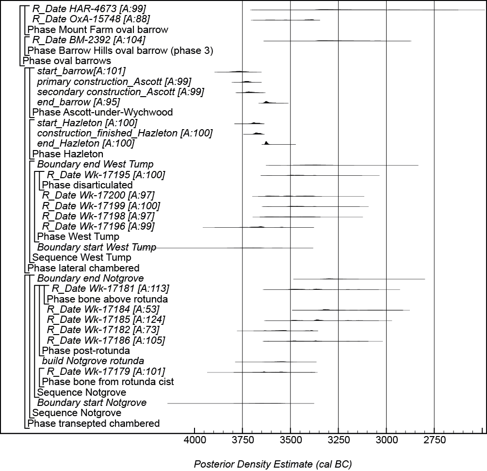
Figure 19: Probability distributions of dates for transepted and lateral chambered long barrows and oval barrows. The format is identical to that for Figure 15. Distributions have been taken from the site models described in detail in Meadows et al. (2007, figs 6–9 (Hazleton)), and Bayliss et al. (2007, figs 3 and 5–7 (Ascott-under-Wychwood)). The structure of the models for Notgrove, and West Tump are derived from Whittle et al. (2011, figs 9.24 and 9.26). The overall structure of this model is shown in Figure 16, and its other components in Figures 17 and 18

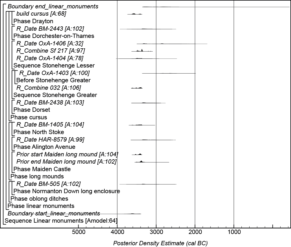
Figure 20: Probability distributions of dates for linear monuments. Distributions have been taken from the site models described in detail in Whittle et al. (2011, figs 4.41–4.45 (Maiden Castle) and 8.3 (Drayton)). The format is identical to that for Figure 15. The large square brackets down the left-hand side along with the OxCal keywords define the overall model exactly

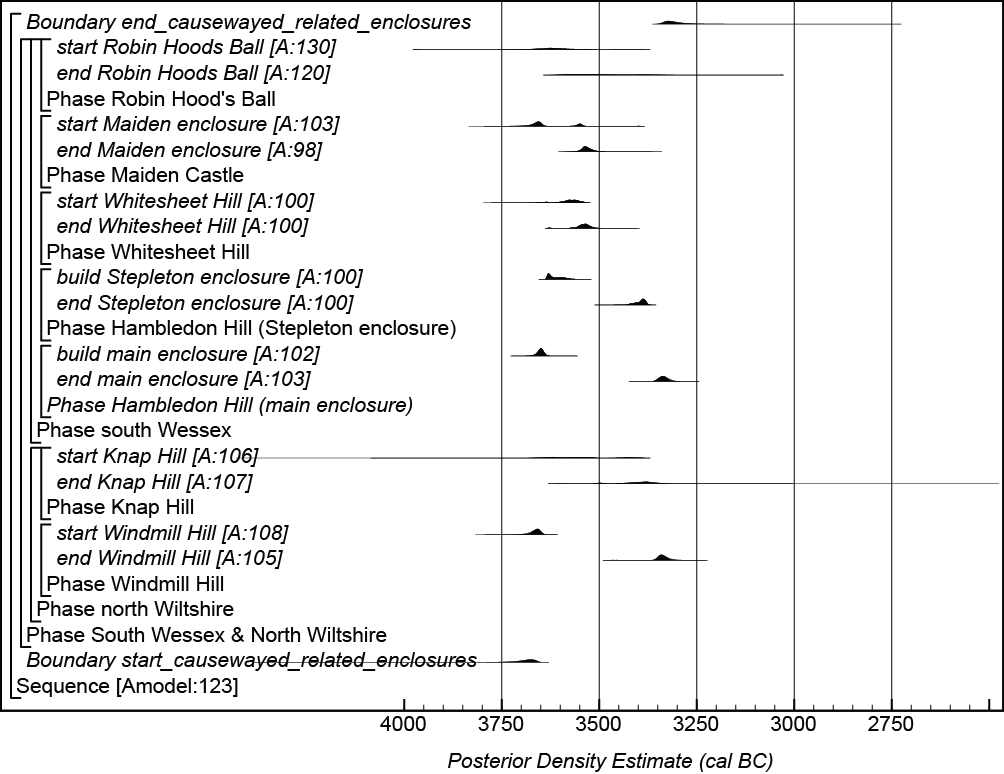
Figure 21: Probability distributions of dates for causewayed and related enclosures from south Wessex and North Wiltshire. Distributions have been taken from the site models described in detail in Whittle et al. (2011, figs 3.8–3.11; (Windmill Hill); fig. 3.25 (Knap Hill), fig. 4.51 (Robin Hood's Ball), figs 4.41–4.45 (Maiden Castle), fig. 4.26 (Whitesheet Hill), and figs 4.7–4.13 (Maiden Castle)). The format is identical to that for Figure 15. The large square brackets down the left-hand side along with the OxCal keywords define the overall model exactly

 PREVIOUS   NEXT   CONTENTS   SUMMARY   ISSUE   HOME