Fig. 11: Excavation areas during the years 1969-1993 (after Mania).
During the excavations of 1969-1993, an area of about 1200m2 was excavated (Fig. 11). In the early years of excavation (1969-1974), the excavation units had irregular shapes. After 1974 squares of 1.5 m became the standard excavation unit (see the table of irregular and regular excavation units now expressed as x-y coordinates).
Fig. 11: Excavation areas during the years 1969-1993 (after Mania).
The excavation squares are numbered consecutively beginning with 1. Within each excavation unit, the finds are numbered starting also with 1. All finds are given a label containing two pieces of information: the number of the excavation unit and the number of the find (a normal label would thus read for example: 105/72, indicating that find No. 72 comes from excavation unit 105). Finds were registered on lists according to their numbers, and many finds were plotted on the excavation plans according to their grid square.
A prerequisite for effective spatial analysis was the creation of a standard grid of 1.5 m squares covering the entire excavation (Fig. 12). Calling one side of each excavation unit 'x' and the other 'y' enables plotting of all single finds as x-y coordinates.
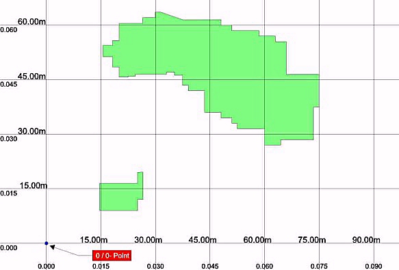
Fig. 12: X-Y coordinates projected onto excavation area - note square size of 15m2 i.e 10 grid
squares of 1.5m.
(also see table of excavation units).
The spatial distribution of the antler finds from Bilzingsleben forms only one aspect within the overall spatial distribution of finds, and only partly reflects the distribution of the other categories. Comparisons with the distributions of other find groups cannot yet be drawn, because the prerequisite x-y coordinates of their respective grid squares are still not available.
Many preliminary density maps were published by Mania (1986a; 1993b) for a wide variety of find groups, including parts of the antler material. New density maps based on antler distribution were prepared for this article in order to explore the evidence further. 2547 finds were included in this analysis. The remaining 273 antler finds from the excavations could not be mapped. The distribution of the finds plotted over the different horizons of the palaeogeographic reconstruction is as follows:
| Chara limestone horizon | 513 finds |
| Pavement | 76 finds |
| Channels below the diluvial fan | 76 finds |
| Diluvial fan sensu lato | 1151 finds |
| Shore terrace + diluvial fan sensu stricto | 731 finds |
Only 76 finds are recorded from the channels below the diluvial fan. A distinction must be made between finds from the diluvial fan sensu stricto (finds that definitely come from the travertine sands of the diluvial fan) and finds from the diluvial fan sensu lato (finds which could either come from the channels below the diluvial fan or from the travertine sands of the diluvial fan). Nearly all finds from the diluvial fan horizon, with travertine sand thickness between 0.1-1m, were not documented with their exact height level. Finds from the Chara limestone horizon, as well as small finds from other facies, have mainly undocumented positions and were randomly spread over the excavation unit from which they came. The midpoints of all plottable finds were expressed as x-y coordinates of the excavated grid square (Fig. 12) and used as the basis for the density analysis.
The density map of all antler finds from all stratigraphic positions (Fig. 13) shows most grid squares containing a minimum of between 1 - 8 finds per square, while two areas included a higher antler density. The first, in the western and central part of the excavation, is divided into two. The second area with frequent antler finds lies to the south. The first area is located in the diluvial fan facies (see figure 1), whereas the latter extends into parts of the pavement area and adjacent squares north of that facies . The pavement facies concentration consists of finds excavated from the Chara limestone horizon. A density map of all antler finds other than those found in the Chara limestone horizon (Fig. 14) does not show the same concentration, still visible however is the diluvial fan facies concentration, as it is also in the distribution of tines, tine fragments and antler cortex fragments from all stratigraphic positions (Fig. 15).
Fig. 13: Density map of all antler finds from all stratigraphic positions.
Fig. 14 (l): Density map of antler finds other than those from the Chara limestone horizon
Fig. 15 (r): Density map of all tines and antler cortex fragments from all stratigraphic positions.
Separate density mapping of tine tips (Fig. 16), medial tine fragments (Fig. 17) and antler cortex fragments (Fig. 18) from all stratigraphic positions confirms that the diluvial fan facies concentration primarily contains tips of tines and medial tine fragments, whereas the concentration adjacent to the pavement area mainly consists of antler cortex fragments, which (as seen above) are mainly concentrated in the Chara limestone horizon.
Density maps for crowns and crown fragments (Fig. 19), fragments of shed antlers (Fig. 20) and fragments of unshed antlers (Fig. 21) from all stratigraphic positions show a more homogeneous distribution over the excavated area.
Fig. 16 (l): Density map of all tine tips from all stratigraphic positions.
Fig. 17 (r): Density map of all medial tine fragments from all stratigraphic positions.
Fig. 18 (l): Density map of all antler cortex fragments from all stratigraphic positions.
Fig. 19 (r): Density map of all crowns and crown fragments from all stratigraphic positions.
Fig. 20 (l): Density map of all shed antler fragments from all stratigraphic positions.
Fig. 21 (r): Density map of all unshed antler fragments from all stratigraphic positions.
Density maps based not on antler morphology, but on grouping material by length - <50mm (fig. 22); >=50mm but <100mm (fig. 23); >= 100mm but <155mm (fig. 24) - were also examined and showed that finds <120mm (Fig. 25) formed the main constituent in areas with higher antler occurrences. The maximum density of finds >= 155mm (Fig. 26), with accumulations of up to 9 finds per grid square, partly coincides with the areas of high antler occurrences (Fig. 13) but some concentrations are found outside those areas.
Fig. 22 (l): Density map of all antler finds <50mm from all stratigraphic positions.
Fig. 23 (r): Density map of all antler finds > 50mm and < 100mm from all stratigraphic positions.
Fig. 24 (l): Density map of all antler finds > 100mm and < 155mm from all stratigraphic positions.
Fig. 25 (r): Density map of all antler finds < 120mm from all stratigraphic positions.
The thickness of travertine sands per grid square was mapped using unpublished data provided by D. Mania. All finds from all stratigraphic positions (with the exception of low values of less than 8 finds per square) were transferred to the map (Fig. 27), showing that a high concentration of antler material coincides with areas of travertine sands at their thickest.
The distribution of finds greater than or equal to 155mm (Fig. 26) is similar to the distribution of antler bases and lower beams of shed and unshed antlers from all stratigraphic positions (Fig. 28). The highest values per excavated square range between 6-9 finds and hardly exceed the lowest number of finds per square of all antler finds in the excavated area. The highest values of this group mostly coincide with squares in the areas of high antler occurrences, and hence where the travertine sand is thickest.
The analysis, particularly the coincidence of maximum sediment thickness with maximum density of finds, confirms that at least for finds <120mm, fluvial accumulation forms part of the site formation process. Furthermore, some kind of sorting can be deduced from the different densities of tips of tines and medial tine fragments in contrast to flat antler cortex fragments. The latter show a distribution similar to that of bone flakes mapped by Mania (1993a, fig. 15).
Since many but far from all of the big antler finds with lengths >155mm (especially lower beams) are also found in large numbers in the diluvial fan facies and in areas with high travertine sand thickness, intentional deposition by hominids cannot be proven by the density plots. Experiments by Stopp (1997) have showed that even low energy fluvial forces are strong enough to transport bone material of similar dimensions to that at Bilzingsleben. The lack of exact stratigraphic origin data for most of the finds from the diluvial fan, which is known to contain small channels running in different directions, prohibits further clarification. It is evident, however, that fluvial accumulation cannot be discounted.
Fig. 26 (l): Density map of all antler finds > 155mm from all stratigraphic positions.
Fig. 27 (r): Thickness of travertine sand and distribution of density categories of all antler finds, apart
from the
smallest density category of 1 - 8 antler finds (see Fig 13).
Fig. 28: Density map of all fragments from unshed and shed antlers from all stratigraphic positions.
© Internet Archaeology
URL: http://intarch.ac.uk/journal/issue8/vollbrecht/en/6.html
Last updated: Thu Aug 10 2000