Probably the easiest and most straightforward method to get a preliminary insight into the spatial relationships within a cemetery is to map the distribution of individual variables stored in the descriptive database. This approach has only limited analytical power but can identify points of interest that may contribute to refining questions previously raised. Two examples of variables having such informative potential will be presented.
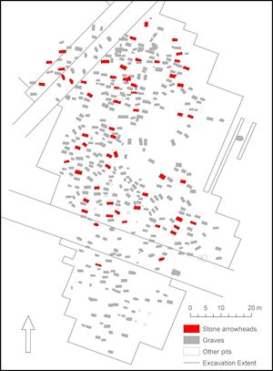
The first example shows where stone arrowheads occur in burial assemblages, disregarding their actual numbers (Figure 7). This draws our attention to the apparent lack of arrowheads in the graves located in the southern part of the site (remember this is supposed to be a later extension of the cemetery). Both central and north areas appear to show a more or less homogeneous distribution of graves containing this typical male grave good.
The second example chosen for this demonstration deals with the depth of grave pits, as they were recorded by the excavators. They measured the depth of every grave from the level reached after the removal of topsoil. The set of measured pits was divided into three groups in the present analysis, the possible spatial clustering of which was then investigated (Figure 8). As the histogram distribution of grave depth values is close to the normal distribution, it seems appropriate to use standard deviation as the natural 'breaking point' dividing the three classes of grave pits. The middle group is labelled 'average' since it includes values concentrated within one standard deviation interval from the arithmetic mean of the whole set (–1σ;+1σ). The values exceeding this range became part of 'outlier' groups. As a result, the subset of average values varies between 66cm and 122cm, a group of extremely shallow grave pits is delimited by the interval of 30–66cm, and the extra deep graves start at 122cm and approach the maximum of 220cm. Somewhat surprisingly, the subsets of very shallow and very deep graves tend to make clearly opposing groups when mapped in the site plan.
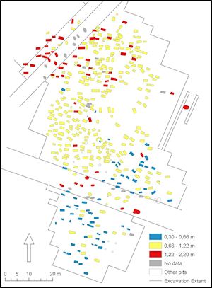
Grave pits that fall into the below-average group cluster in the southern area, while the above-average graves concentrate mainly in the northern part. Average values are highly typical for the middle section of the cemetery, although they can also be found in the north and south borders, albeit less often.
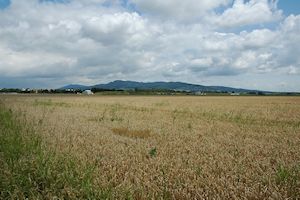
The interpretation of this intriguing phenomenon is not straightforward. Natural factors, such as a sloping terrain, are ruled out because the site is situated on a plain, recently used as an airfield (Figure 9). According to the topographic map the flat surface is gently sloping in an east-west direction; it is therefore difficult to imagine that, for instance, soil accumulations could have caused the differences in the grave depths measured in the north and south ends of the site. The methodology used in the process of excavation recording was not explicitly described in the publication (Ondráček and Šebela 1985); however it seems to be standardised, at least for the great majority of graves excavated by Ondráček. The original (unpublished) excavation report mentions, however, that in the southern part of the site the topsoil layer had been removed and the surface levelled in the process of airfield construction. Although this event, as well as the former digging of drainage canals, might have caused some inconsistencies in the recorded measurements, it seems improbable that it would fully account for the overall pattern found in the data. The trend of decreasing grave depths from north to south might have a chronological basis; however, we should keep in mind that this is only a general thesis, valid 'on average', when larger zones of the site plan are compared. Individual departures from the rule do exist, namely a few 'oversized' graves in the east and south-east border of the site, most probably intended as signs of the non-standard character of some graves (high-status burials).
It is important to realise that distribution maps, as they have been applied in archaeology, communicate facts whose contemporaneity is uncritically assumed. Even though they look like snapshots, capturing a moment in time, they usually represent events that happened over a broader interval of time. There is always some danger of misinterpreting patterns of temporal development as patterns of functional structures of human culture. In the case of Holešov cemetery, most materials and artefact types are distributed across the whole cemetery and do not define any clear spatial structures, at least when mapped on a presence/absence basis.