3 Bayesian wiggle-matching (intuitive)

Radiocarbon dating is a technique for dating organic samples (e.g. see Bowman 1990). However, for archaeological research this is frequently not good enough: the archaeological context under study is in fact what needs to be dated, and not just the individual samples themselves. Bayesian radiocarbon calibration was developed precisely to deal with this problem (e.g. see Buck et al. 1992 or Christen 2002 for a review). One particular example of this is the dating of a log or timber, using radiocarbon (indeed, if available, absolute dendrochronological dating could be used instead; see http://web.utk.edu/~grissino for a comprehensive resource). Chunks of tree-rings may then be sampled and sent for radiocarbon dating. However, we already know that the calendar ages for the chunks are ordered in the calendar scale and, moreover, by counting the number of tree-rings separating them it is possible to calculate the differences in calendar ages between samples. This information could be used both in order to calibrate all of the radiocarbon dates and produce an agreed dating for the log, instead of each determination producing a separate date. Wiggle-matching attempts to do that and Bayesian wiggle-matching uses an established statistical theory, namely Bayesian statistics, to solve the problem.

Bayesian statistics is a theory for inference and decision making, developed mainly in the last century, that advocates an alternative paradigm to tackle the problem of inference. It differs from more traditional ways of understanding statistics, such as the classical (or frequentist) approach. It is not the purpose of this article to make a thorough exposition of Bayesian statistics. The reader is referred to Howson and Urbach (1993) for a more philosophical (epistemological) explanation, to O'Hagan (1988) for a simple, mathematical, exposition and to Bernardo and Smith (1994) for a complete exposition of the mathematical theory. An excellent introduction to Bayesian ideas applied in archaeology may be found in Buck et al. (1996).

The main criterion for interpreting the output of a Bayesian analysis (e.g. Bwigg output), is what is understood by 'probability'. Probability in this context is defined as 'the numerical measure of [a person's] degree of belief in [an event]' (Howson and Urbach 1993, 76). Commonly, in the Bayesian jargon, the person refers to you (and thus gives rise to the term 'subjective' statistics), although we could also think of person as a working group in an agreed context. In any case, probability is regarded as a measure for degrees of belief and thus conditional on information, models and data, used and/or currently available. Bayesian statistics then provides (by the use of Bayes' theorem) a means of updating degrees of belief in relevant events (probability) in the light of new data. Posterior (a posteriori, after having the data) probabilities are then obtained. The Bayesian paradigm has proven very useful in the analysis of archaeological data since it allows for the inclusion of several forms of (a priori) information in the analysis, commonly a crucial feature in archaeological investigations (see Buck et al. 1996).

With respect to the output of Bwigg, we have the posterior distributions in Figures 1 and 2. These probability distributions represent the degree of belief about the value for the event θ₀ (the event that fixes the floating chronology - see section on software usage and technical issues). The two distributions differ since the model used is different. Figure 2 includes an error term to account for the error observed in the calibration curve, whereas Figure 1 excludes this error. For interpretation purposes, Figure 1 will be used. Note that the highest point is at 2191 BP, with a probability of nearly 0.18 (18%). If a single year had to be chosen for θ₀, then it would be 2190 BP. However, there is no reason whatsoever for choosing one year only. An interval of time could be selected – for example 2170-2210 BP. In that case, we know with nearly a 100% certainty that θ₀ belongs to this interval, conditional on the fact that there are no errors in the calibration curve, the normal model assumed, the data, and the time span used (the prior distribution; we used the span 2,600-2,000 years BP). Note also that we are not restricted either to producing a (confidence or probability) interval at any level or to choosing a single calendar year. The posterior distribution itself has far more information than point or interval estimates and lends itself for richer, although perhaps more complex, interpretations. A table with the numbers generating Figure 1 (and other figures) may be downloaded from the corresponding Bwigg output page (see software usage). This table may be used for more precise accounts of the posterior distribution. The reader is invited to perform a similar interpretation exercise with the more convoluted posterior distribution depicted in Figure 2 (including the errors in the calibration curve).

Figure 3 presents the floating chronology, with the radiocarbon determinations, superimposed on the relevant part of the calibration curve. The chronology is fixed at (θ₀=) 2190 BP, the year with the maximum probability for the posterior in Figure 2. That is, according to our current knowledge (time span provided), best model (errors in the curve) and data, the single most certain point for θ₀ (however, as stated above, it is not necessary to choose one single point to fix the chronology). This superimposition illustrates the resemblance between the wiggles formed by the floating chronology and those of the calibration curve (thus the term wiggle-matching). The remaining output to be interpreted relate to the posterior probabilities, in the outlier section. This is what happens next.

Outliers

In statistics the term 'outlier' is assigned to data points outside the main range of the rest of the data, of spurious or conspicuous origin, abnormal or difficult to explain according to standard theories or, simply, wrong or misleading. Outliers are a constant concern in radiocarbon dating (see Scott et al. 1990). However, the term outliers cannot be employed unless referred to a context, a data set and models used (see Christen 1994b for a more in-depth discussion). In the case of wiggle-matching, it is radiocarbon dates that stand out of the floating chronology that are important, even accounting for their intrinsic variability (the standard error reported σ_j), and the errors in the calibration curve. For those determinations, an additional shift in the radiocarbon scale is used in order for them to be correctly fitted in the floating chronology. It is then possible to calculate (by a numeric approximation called MCMC, see technical section) the probability that each determination needs such a shift. This is what is called the posterior probabilities of each determination being an outlier (see technical details). A priori, there is a 5% probability for each determination being an outlier. Note also that the errors in the calibration curve are taken into consideration to perform the outlier analysis.

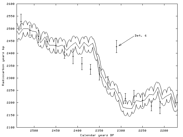
As an illustration, take the data set in Table 1 and change determination j=6 (lab. number 4079) from 2247 to 2427 BP, keeping σ₆ = 25. If Bwigg is rerun, the posterior probability of this determination being an outlier is now more than 0.9 (Bayes factor of more than 18, see below). The determination is clearly detected by the outlier method as standing out of the chronology. As an illustration, see the match given by Bwigg in Figure 4.

Figure 4: Data in Table 1 changing determination 6 (from right to left) to 2427±25, simulating an outlier. The floating chronology is fixed at (θ₀ = 2210 BP as provided by Bwigg. The relevant part of the calibration curve are also presented, with the estimated standard errors in the curve

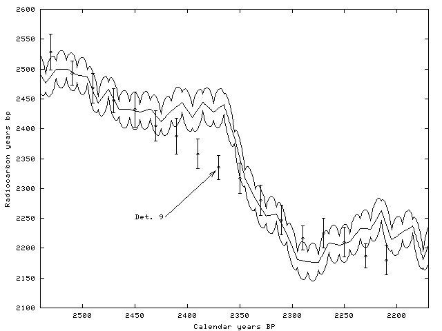
Bwigg also presents the 'Bayes factors'. These are the posterior probabilities divided by the prior probabilities (0.05) of each determination being an outlier [1]. This factor represents the number of times it is more certain that the corresponding determination is an outlier. For example, going back to the original data set in Table 1 the highest Bayes factor in Table 2 is 2.11, corresponding to determination j=9. This means that the probability of this determination being an outlier doubled a posteriori. However, surprisingly, looking at Figure 3, this determination (the 9th from right to left) falls nicely within the calibration curve. Nonetheless, we must remember that the match presented in Figure 3 is only one possibility, accumulating only 7% of probability (see Figure 2). There is some variability for probable values for θ₀, and given the steep slope of the calibration curve where determination j=9 is positioned, this determination might end up being slightly out of the chronology (note that, in fact, the corresponding posterior probability is only 0.1). For example, an alternative probable match would be θ₀ = 2210, only 20 years earlier than the match provided by Bwigg (= 2190). This corresponds to the third most highest peak in the posterior distribution presented in Figure 2. In Figure 5 we present the floating chronology using this match. Determination j=9 may now be regarded as slightly out of the chronology. A threshold may be established for outlier posterior probabilities beyond which determinations may not be considered in the chronology. In any case, the recommendation would be to report this threshold and all removed determinations.

Figure 5: Data in Table 1, fixing θ₀ = 2210 BP; the third highest peak in Figure 2.

Footnote 1: The reader should note that Bayes factors and posterior probabilities may be combined to produce posterior probabilities corresponding to other prior probabilities, besides 5%. Given the posterior probability P_o for a determination, corresponding to a prior of 5% (the output of Bwigg), and its corresponding Bayes factor BF,

		   Q*p
		__________
		Q*p + (1-p)

would be the corresponding posterior probability using a prior probability of p; where Q = BF/{(1-P_o)/0.95}.

© Internet Archaeology URL: http://intarch.ac.uk/journal/issue13/2/3int.html
Last updated: Thu Jan 23 2003