It would be possible to plot the results of factor analysis on the site plan but unfortunately this is not really helpful. Some spatial trends would be recognisable as they more or less follow the patterns described in previous sections, mixed with much noise stemming from the fact that demographic groups from different time periods are to a large extent intermingled in the funerary area. The logical consequence is that spatial patterns representing individual factors are not clearly manifested in geographical space. Therefore, when we change the frame of reference from geographical coordinates to coordinates that correspond better to the latent order hidden in our formal variables, we may get more intelligible results.
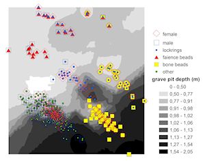
Following the line of thought suggested above, we can prepare maps with a non-geographical frame of reference (although the geographic space may sometimes be indirectly reflected in their content). A 'map' in Figure 13 is defined by a coordinate system based on the so-called factor scores of factors #1 and 2, which are one of the outputs produced by factor analysis. This image can be regarded either as a two-dimensional statistical plot explaining 32 % of total variance (18 + 14 % respectively for each factor) or as a map of fact space in one specific projection. Similar outputs can be created in statistical software packages but many of them are not that user-friendly and, unlike the quickly evolving GIS software, are not as open to modifications and experiments in visualisation. As usual, the best way is simply to combine both and be creative – where one software fails, the other succeeds. In the case presented here, factor analysis was computed in statistical software (Statistica 6) and final visualisation was done in GIS (ArcGIS 10).
How can this graphical representation be interpreted? The spots marked by different symbols represent individual burials. Their distribution now does not correspond to their spatial position, but to the degree of their overall similarity or dissimilarity given their sets of grave goods and dimensions of grave pits (in other words it is their position in the formal part of fact space). A distinctive ordering of burials that are accompanied by ornaments such as beads and hair ring ornaments made of copper wire is well displayed in this picture, showing the structural distinction between the burials with faience beads and those with bone beads. Each existing combination in the category of ornaments (bone beads, faience beads, copper hair ornaments) is depicted as a compact cluster of similar burials.
The background of this map displayed as grayscale gradient may resemble a digital elevation model (DEM) commonly used in GIS (Chapman 2006; Shekar and Xiong 2008). However, in this case it is an interpolated surface computed from a set of grave depths by the Inverse Distance Weighting method (Conolly and Lake 2006, 94-7). As a result, we can see an internal organisation in our data. Bone beads show a strong tendency towards deeper graves (darker bands) and faience beads towards shallow graves (located in zones of lighter grey). We have already learned that shallow graves are typical of the south part of the site and deep graves are frequent in the north part. This means that one important aspect of the ordering of burials in the geographic space is also present in this abstract model. But, unlike the conventional maps, a particular spatial attribute is not used here as the frame of reference, but is latently present as a hidden variable correlating with the thematic content of the map.
Although this may seem a completely inverted concept of conventional cartography, I want to argue that by the application of this approach it is possible to produce very helpful maps that articulate clearly the internal structuring of archaeological data. When used in combination with a well-organised theoretical background they have a great potential to describe latent structures of large datasets and considerably improve our understanding of their complex relationships.
The previous map can be reworked in a couple of minutes into another projection that refers to a different pair of factors, this time factors #3 and 4 (Figure 14). It logically follows that the marks in the content of this 'map' are now organised in accordance with these axes of variability (these two factors explain 22 % of total variance, 12 and 10 % each). Cattle ribs and stone blades clearly stand in opposition (occupying the upper and lower part of the diagram respectively), because they usually do not occur together in burial assemblages. Stone arrowheads can accompany either of these two variables, exceptionally both (in one case) or neither of them, which is a relatively common situation. We must be aware that this overview does not list full combinations of grave goods that exist in reality, but it picks up only the group of strongly correlated variables (positively or negatively), those that constitute the extracted factors #3 and 4. It means that burials that show only one type of grave good in the diagram can in fact be combined with other types of grave goods, which are not characteristic for factors #3 or 4. Some of those types can belong to other factors (i.e. intentional components in burial assemblages that may convey a particular message in burial symbolism) or they are so rare that they do not contribute to statistically significant correlations and therefore are omitted in this article. Here I focus only on the most frequent traits, which produce strong structures and interrelationships, and are repeated many times in the funerary ritual across large parts of the cemetery (see Borić 2003 for the concept of repetition/recapitulation of ritualised practices as the means of social mnemonics in settlement context). I will return to this point below.
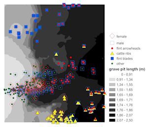
The interpolated surface in the background indicates variations of grave lengths (again using the Inverse Distance Weighting method) and it is not hard to observe that arrowheads are likely to be found in longer grave pits (in darker zones to the right of the picture). This relationship between long grave pits and stone arrowheads is strong enough to be taken as an intentional feature of burial customs. When we distinguish burials of males and females by the side on which the deceased lies (Figure 14), we can see that it is in the first place the difference between graves of males (which tend to be longer) and females (which are typically shorter, or at least do not reach to exceptional lengths over 2m as do some male graves). It is difficult to read something meaningful from the distribution of short graves as we would have to filter out the graves of children, which are normally shorter than graves of adults.
I have shown elsewhere (Šmejda 2003b, fig. 8) that despite the broad overlaps between both sexes, the male graves tend to be longer than female ones in all age groups. It does not seem to be simply a functional trait, reflecting the difference in height between the sexes. In inhumations of flexed bodies such differences are negligible and it is apparent that graves were frequently dug a great deal longer than would be necessary for placing a body. Therefore we may assume that the length (and width) of the grave is charged with cultural significance and some burials were afforded a grave excessively larger than necessary. The depth and volume of graves understandably co-vary with length and width, but length is clearly the leading metric, correlated most strongly with gender and grave goods; other grave dimensions probably followed, more or less closely, the scale defined by length. It is worth repeating that stone arrowheads were found normatively in extra-long grave pits, accompanying bodies placed on their right side (males). It seems to be not just an expression of gender but also of special social standing.
Further experiments led by additional research questions can enrich this picture with finer details. It should be clear by now, however, that these results are structural models of mental concepts that once commanded burial rituals. We see that several types of burial goods were gender specific, though with some overlaps. Perhaps more surprisingly, the dimensions of grave pits were closely related to the content of burial goods assemblages and indications of temporal and spatial development were also included in the presented models. Such graphic representations of the past symbolic systems as reflected by the empirical record can help to explain the main principles of the ancient cemetery organisation with its structural oppositions, smooth gradients, and multi-faceted meanings.
These patterns could not be detected if the burials were individualised to a high degree by attributes referencing unique combinations of personal features, complex life histories etc. The case seems to be quite the contrary despite a certain amount of variance: the burials follow strict rules of burial ideology that was maintained by repetitive stylisation of individuals into a limited number of social roles, referring to and making citations of many other individual interments. The material culture and funerary customs slowly evolved during the temporal and spatial development of the site, but it was the tradition and continuity that governed them, not dynamic innovation and bold experiments in mortuary display. There was certainly room for highlighting status and for some personal expressions as witnessed in the non-identical combinations of ornaments and rare miscellaneous artefacts included in grave assemblages. However, the underlining principles were strict and it seems that burial identity in the Early Bronze Age was still rather collective and relational than freely individualised (Bruck 2004).
Departures from the norm are not frequent and pronounced at the site of Holešov but should be noticed and duly analysed. As they are not repeated on a larger scale, they could not be properly embraced by this study based on mapping regularities, mnemonic repetitions and main cognitive categories related to funerary rituals. These provide indispensable guidelines that allow us to navigate in the structure of mortuary behaviour and prepare the ground for a more nuanced narrative, investigating the material metaphors used in burials, role and type of agency involved, and the significance of details that remain beyond the scope of the formalised methods used in this article.