A commercially available GIS package, Esri ArcGIS 9.x, was used by the Stonehenge Riverside Project Data Manager to manage and manipulate the spatial data gathered by the project. This section will document the methodologies used to export the different layers that were used within Seeing Beneath Stonehenge, as well as identifying other alternative methodologies that could now be used.
Trench outlines were one of the first data layers to be exported into Google Earth. The data archive contained a number of iterations of the same trenches, as different parts of the same trench had been excavated during different seasons. Using ArcGIS, all of the outlines were exported to a new geodatabase and the maximum extent of each trench was then digitised. New attribute fields were added to provide further information about the trench history, including excavation start and finish year, the site code and a summary of the main discoveries within. The embedding codes for individual photos of each trench were also included from Flickr, allowing images to appear underneath the descriptions once these trenches had been selected within Google Earth.
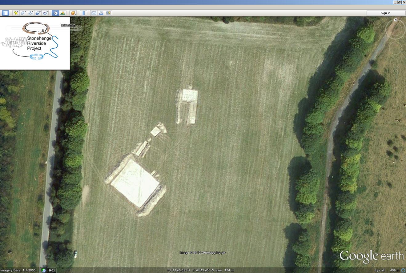
To export these features into Google Earth, an extension downloaded from the Esri Support Centre website was installed and used to convert the geodatabase into KML format. This extension was developed by the City of Portland, Bureau of Planning and allowed for the export of any point, polyline, or polygon dataset, in any defined projection, to KML (Esri 2010). During this process, a number of export options were available. The most critical of these was the Coordinate System Transformation Method, where the GIS layer was converted from British National Grid, OSGB_1936 into the coordinate system used by Google Earth, Simple Cylindrical projection with a WGS84 datum. When no transformation method was used, a vertical and horizontal difference was recorded of 100m and +50m respectively, owing to different coordinate values on the ground in the input and output geographic coordinate systems. Testing the various transformation methods established a maximum horizontal inaccuracy of 2.5m and a maximum vertical inaccuracy of 16m. An assessment of the accuracy of the different transformation methods could be undertaken owing to the 2005 historical imagery in Google Earth, which showed a number of open excavation trenches. By overlaying the differently converted trench outlines, measurements could be made to determine the most accurate. The chosen transformation method was OSGB_1984_Petroleum, which had a horizontal inaccuracy of 0m and a vertical inaccuracy of +0.5m (Figures 6 and 7).

Further options enabled the export of a KML Layer Description and Feature Descriptions. Information from the geodatabase attribute fields were used to create the latter, which included the Trench ID, Site Code, excavation summary and embedded photos. The layer was automatically added to Google Earth and saved as a KML file (Figure 7).
In recent years the further development of ArcGIS has seen this process become less complicated with the introduction of the 'Export to KMZ' tool. In addition, open source software such as Quantum GIS also provides an alternative to exporting shapefiles into Google Earth. One consideration of these latter developments is that previously it was possible to select which attributes to transfer, as well as their order. Currently both software systems automatically transfer all attributes, and therefore a bespoke shapefile would need to be created to define both content and order of display.
Once the transformation parameters for the trenches had been determined, the same processes could then be applied to convert archaeological features. To create this information, a number of excavation plans were geo-referenced and digitised within ArcGIS. Once completed these then had information added to them within the attribute tables (e.g. feature type and associated context), and were exported through the process described above (Figure 8).

Earth resistance and fluxgate magnetometer surveys were conducted over several sites during the Stonehenge Riverside Project including Durrington Walls, Larkhill, the Palisade, the Stonehenge Avenue, Bulford, the Greater Cursus and West Amesbury. The results of these surveys were archived as georeferenced (British National Grid) tiff images (GeoTiffs). Theoretically, it was possible to import these images directly into Google Earth as GeoTiffs. However, these do not display background layers as transparent, which was important as many geophysical plots are irregularly shaped, and areas of 'no data' would show up as white. Therefore, a different approach was used. Using Corel Paint Shop Pro Photo X2, each geophysical plot was cropped to the survey edge. The cropped image was then saved as Portable Network Graphic (PNG). The PNGs with areas of 'No Data' were set to display as transparent, letting the underlying imagery show through. However, this process lost the georeferencing information associated with the images. To re-locate them within Google Earth, the outline of the survey data was traced as a polygon shapefile in ArcGIS and exported as a KML file, using the same OSGB_1936 to WGS84 transformation method outlined in section 3.2.1. The modified PNG image was then added to Google Earth using the 'Add Image Overlay' tool. The image was then positioned to match the appropriate polygon shapefile. Once complete, the image was saved as a KML file within Google Earth. Again, new versions of ArcGIS 10 have allowed this process to be completed faster using the 'Export Map to KMZ' tool. There are, however, some issues with this approach when it comes to the resolution of the exported image, and the original method described above provides an improved end result.