![]()
![]()
![]()
![]()
Bwigg is an interface to the general purpose Bayesian calibration software mexcal. After formatting the input data, Bwigg collects the output from mexcal and calls the graphics software gnuplot to create the figures. Bwigg then creates an HTML document with an outline of the results, with links for output file retrieval.
An interface for mexcal, including several features for Bayesian calibration (not including wiggle matching, however), may be found in BCal. Other software for radiocarbon calibration includes OxCal, Cal25 and CalPal. Access Bwigg at http://www.cimat.mx/Bwigg (this will open in the frame below. Alternatively, select this link to open the site in a new window). Reading all the text in the introductory page is strongly recommended.
It is assumed that the set of radiocarbon determinations to be calibrated form a floating chronology. First, the determinations should be sorted starting with the latest (youngest) sample in the calendar scale. For tree-rings, this would be the outer-most sample in the sequence. Second, the event of interest should be established. For example, suppose the bark was not radiocarbon dated (say, 30 tree-rings until the border of the log), but the event to be dated is when the tree was felled. In this case the age for the first sample, θ1, is 30 years before the event to be dated. Therefore, using years Before Present (BP; taking as the 'present' the year AD 1950), should be
In such a case α1 = 30 should be set. The same should be done for the rest of the determinations, to complete a list such as the one presented in Table 1 (although for the data set in Table 1, θ0 = θ1, i.e. α1 = 0).
| j | αj | r.c det: yj ± σj | Lab. Number |
| 1 | 0 | 2180 ± 25 | 4084 |
| 2 | 20 | 2187 ± 20 | 4083 |
| 3 | 40 | 2210 ± 25 | 4082 |
| 4 | 60 | 2225 ± 25 | 4081 |
| 5 | 80 | 2217 ± 20 | 4080 |
| 6 | 100 | 2247 ± 25 | 4079 |
| 7 | 120 | 2280 ± 25 | 4078 |
| 8 | 140 | 2317 ± 25 | 4077 |
| 9 | 160 | 2335 ± 20 | 4076 |
| 10 | 180 | 2358 ± 25 | 4075 |
| 11 | 200 | 2387 ± 30 | 4074 |
| 12 | 220 | 2405 ± 25 | 4073 |
| 13 | 240 | 2432 ± 30 | 4072 |
| 14 | 260 | 2447 ± 20 | 4071 |
| 15 | 280 | 2468 ± 25 | 4070 |
| 16 | 300 | 2493 ± 20 | 4069 |
| 17 | 320 | 2528 ± 30 | 4068 |
Table 1: Radiocarbon determinations for the Ulandryk 4 kurgan, Altai Mountains, southern Siberia, dendrosample 19116 (see Slusarenko et al. 2001). In this case θ0 = θ1 (α1 = 0). The laboratory is the Radiocarbon Laboratory of the Institute of Geology, Siberian Branch of the Russian Academy of Sciences in Novosibirsk (standard liquid scintillation counting).
Table 1 is taken from Slusarenko et al. (2001). A log found in a burial place in southern Siberia, belonging to the Pazyryk culture, was analysed. The tree rings were sub-divided into groups of 20 rings each, and seventeen samples (340 rings counted from the centre), were selected for dating, as shown in Table 1 (see details in Slusarenko et al. 2001).
The next step is to access the data input page of Bwigg. A name for the project (task) for Bwigg should be selected. It is recommended that a name characteristic of the dating study is selected. For example, for the data in Table 1 'Ulandryk' was chosen. Next, the data should be entered. The first line, and only the first line, is available (and should be used) for a comment. This line may be used for a short description of the data. Exceeding the width of the input window is not recommended. The data come next. Each line corresponds to one radiocarbon determination. The format for each line is as follows:
The data may first be typed in a plain text editor (e.g. Notepad in Windows, for example, but not Word), and then copied and pasted into the input window. The data from Table 1, ready to be pasted into the input window look like this:
Ulandryk 4 kurgan, Altai Mountains, southern Siberia, dendrosample 19116.
  0	2180 ± 25	4084
 20	2187 ± 20	4083
 40	2210 ± 25	4082
 60	2225 ± 25	4081
 80	2217 ± 20	4080
100	2247 ± 25	4079
120	2280 ± 25	4078
140	2317 ± 25	4077
160	2335 ± 20	4076
180	2358 ± 25	4075
200	2387 ± 30	4074
220	2405 ± 25	4073
240	2432 ± 30	4072
260	2447 ± 20	4071
280	2468 ± 25	4070
300	2493 ± 20	4069
320	2528 ± 30	4068
The last step is to provide a period of time (early and late boundaries) for calibration. This constitutes the a priori distribution for θ0 (see Bayesian wiggle-matching), which is uniform within the early and late boundaries. Although a very wide range may be used, it is strongly recommended that all available knowledge is incorporated, not including the current radiocarbon determinations, to give an educated guess for this period, thus making the range as short as possible (remember that Bwigg only uses years BP). The data are now sent with the send button. Note that a 5% a priori probability is used for each determination being an outlier; see Outliers for details.
After a short processing time, the output report page shows up in your browser. First of all, go to section 4 of the report (Outlier analysis) and write down or copy some or all of the posterior probabilities given. Go back to the input page and re-send the data. The posterior probabilities in the refreshed calculations should be roughly equal to the first calculations. These probabilities are numerically approximated using a simulation method (called MCMC; see technical section). Problems may arise if the time span (early and late boundaries) given to Bwigg is far greater than the span of the posterior distributions (Figures 1 and 2). After some assurance that the approximations are correct, you may turn to analyse the results (note that the posterior distributions, Figures 1 and 2 in the Bwigg report, are calculated exactly).
The results are given in the output page. Here the posterior distributions are reproduced in Figures 1 and 2, not considering and considering the errors in the calibration curve respectively. Also, Figure 3 presents an illustration of the best match obtained. Moreover, the shift-outlier probabilities are presented in Table 2. Of course, the posterior distributions and graphs in Figures 1, 2 and 3 need to be correctly interpreted, together with the posterior probabilities in Table 2. The reader is referred to the intuitive section for a more general explanation and to the technical section for greater detail.
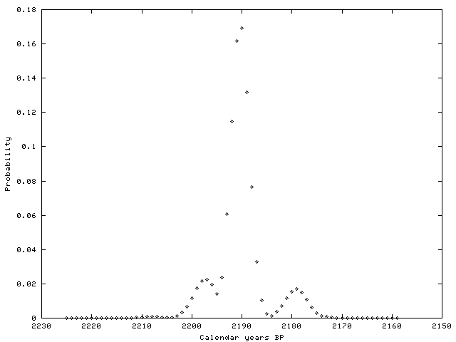
Figure 1: Posterior distribution for θ0, for data in Table 1, not considering the errors in the calibration curve
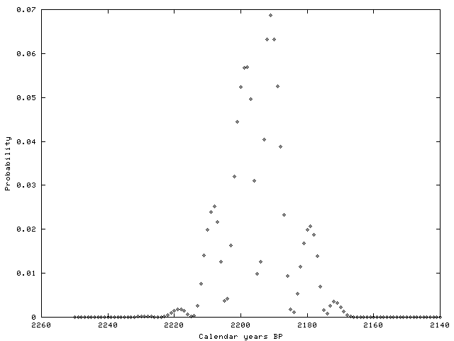
Figure 2: Posterior distribution for θ0, for data in Table 1, considering the errors in the calibration curve
The output explained here is the only output produced by Bwigg. In section 5 of the output page the files produced by Bwigg may be downloaded. These include the figures in png format, which is compatible with nearly all popular word processing packages and may be directly included in your papers. Also, in the compressed (.zip) file there are lots of configuration files, the data file (.dets) and tables in ASCII format defining Figures 1, 2 (.hist files) and 3 (combining .ccur and .dets files). These files may be useful if you want to create your own figures; otherwise downloading the compressed file is not recommended. (For example, the ASCII tables may be imported into Excel to produce customised versions of the figures produced by Bwigg; see Figure 5.)
| j | Lab. No. | Post. Prob | Bayes Fac. |
| 1 | 4084 | 0.0467 | 0.934000 |
| 2 | 4083 | 0.0661 | 1.322000 |
| 3 | 4082 | 0.0353 | 0.706000 |
| 4 | 4081 | 0.0313 | 0.626000 |
| 5 | 4080 | 0.0435 | 0.870000 |
| 6 | 4079 | 0.0635 | 1.270000 |
| 7 | 4078 | 0.0529 | 1.058000 |
| 8 | 4077 | 0.0466 | 0.932000 |
| 9 | 4076 | 0.1057 | 2.114000 |
| 10 | 4075 | 0.0988 | 1.976000 |
| 11 | 4074 | 0.0432 | 0.864000 |
| 12 | 4073 | 0.0350 | 0.700000 |
| 13 | 4072 | 0.0292 | 0.584000 |
| 14 | 4071 | 0.0341 | 0.682000 |
| 15 | 4070 | 0.0323 | 0.646000 |
| 16 | 4069 | 0.0360 | 0.720000 |
| 17 | 4068 | 0.0384 | 0.768000 |
Table 2: Approximations obtained for the posterior probabilities and Bayes factors for each determination being an outlier.
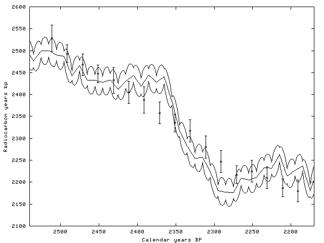
Figure 3: Data in Table 1, fixing
θ0 = 2191 BP; the best match according to Figure 2. Also the relevant part of the calibration curve is presented, with the estimated standard errors in the curve, to appreciate the wiggle match.
![]()
![]()
![]()
![]()
© Internet Archaeology
URL: http://intarch.ac.uk/journal/issue13/2/2usage.html
Last updated: Wed Jan 22 2003