Figure 2: Example of the Vector conversion model for the Currency (Cu) Medieval (Me) ADI process
In this section, the aim is to present the technical detail behind the process of creating the ADI for each dataset, and to discuss how these ADIs were used to create the DC ADIs.
The project used ESRI's ArcView GIS version 3.3 with the extension Spatial Analyst version 2.0. The Extension Grid Machine 6.53 was also used. For the manipulation of data, Microsoft's Access 2003 was used, and some operations were carried out using Excel 2003.
To fulfil the aims of the project, the stray finds needed to go through a number of processes. These can be broken down into four main phases, which will be examined in turn. The four phases were:
Apart from the artefact data, all the GIS data which was not generated by the project came from NYCC, such as the parish and county areas shown in various figures, and the vector mapping. All the NYCC artefacts data was exported from the Exegesis software HBSMR version 3.06 using the XML export function shipped with the program. After data cleaning, there remained 56 stray finds records from the NYCC HER for the project area. The PAS Scheme very generously provided me with all their data for North Yorkshire. After data cleaning, there remained a total of 117 records for the project area.
Once the data were prepared, they had to be included into the GIS in the appropriate format for the ADI process.
There were basically four precision levels that the data could be entered at:
Within each of these tables the appropriate fields need to be created to allow data to be entered. This was done manually. To help with the model creation process, a naming convention was created for the fields. The basic convention was that the name would have two elements, with two letters representing the type of data and two letters for the period. So, for example, data from the Armour and Weapons category from the Early Medieval Period would have the code AwEm; data from the Currency category from the Medieval Period would be CuMe. A full listing of the codes chosen is given in Appendix 3 of the Dissertation.
Once the data had been entered into the appropriate tables, the actual processing of the data to form the ADI could begin. The first process was to create the raster data from the vector data.
Figure 2: Example of the Vector conversion model for the Currency (Cu) Medieval (Me) ADI process
Essentially, this involves converting data from the format in Figure 5 to that shown in Figure 6.
This was done using the standard vector conversion functionality within ArcView. Again a naming convention was designed for the themes created, which contained three elements - the two already discussed above plus an additional one showing the precision of the dataset. So, for example, data for Currency of the Medieval period for 100 metre accuracy would be called Cu100Me. In each case the vector data was converted into raster grids of 100 metre square size.
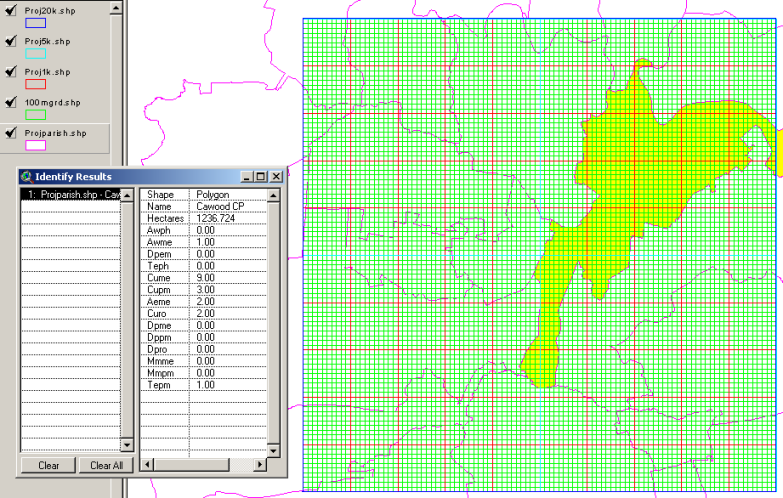
Figure 3: Screen shot from ArcView 3.3 showing the vector data for the highlighted civil parish of Cawood
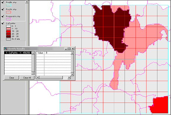
Figure 4: Screen shot from ArcView 3.3 showing the raster data for the CuMe ADI process for the project area
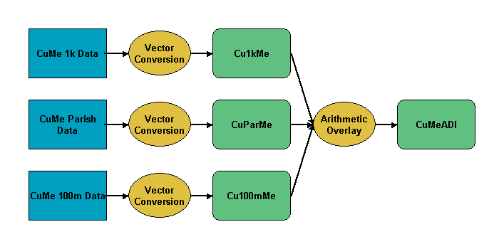
Figure 5: Example of the dataset specific ADI model for the Currency (Cu) Medieval (Me) ADI process
Once all the raster data had been created, the dataset specific ADI could be created (i.e. separate ADIs for e.g. Medieval Armour and Weapons; Post-Medieval Currency, Medieval Currency etc.). The naming convention for this was the same as for the vector conversion, with the addition of a suffix of ADI. So, for example, the ADI for Currency of Post-Medieval date would be named CuPmADI.
The process of creating the overlay involved adding together the different raster layers, using the Arithmetic Overlay function in Model Builder. (This process is shown graphically in Figures 8, 9, 10 and 11.) This allows the different themes to be weighted as they were added together. The weighting was used to reflect the precision of the artefacts' location based on the original size of the polygon.
The hierarchy which was used to determine the weighting was based on the relative sizes of the areas and was as follows: 100 metre square (base unit); kilometre square; parish and then quarter sheet. The logic of this was that the average size of parishes was calculated to be 894 hectares, which put them in between the 100 hectares of a kilometre square and the 2500 hectares of the quarter sheet. For simplicity, all parishes were weighted the same regardless of size.
Once the ADI had been calculated, the theme was saved as a grid theme with a similar naming convention to that mentioned above, but with the suffix of the term ADIGrd. So, for example, the ADI for the Currency class of the Medieval period was given the name CuMeAdiGrd.
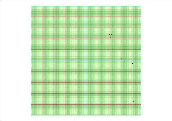
Figure 6: The raster grid created for the 100 metre precision level for the Currency (Cu) Medieval (Me) ADI process
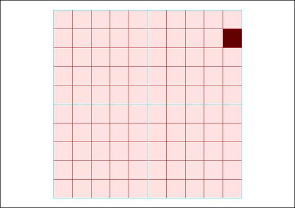
Figure 7: The raster grid created for the kilometre precision level for the Currency (Cu) Medieval (Me) ADI process
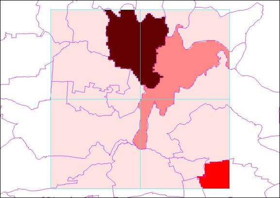
Figure 8: The raster grid created for the parish precision level for the Currency (Cu) Medieval (Me) ADI process
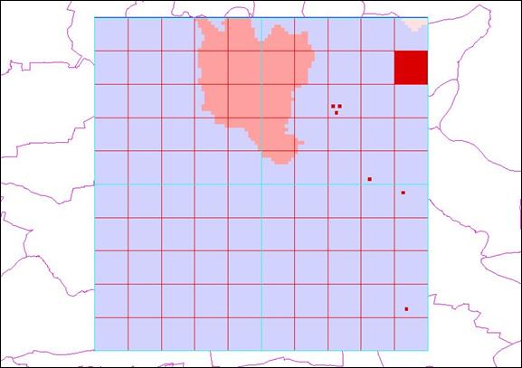
Figure 9: The Currency (Cu) Medieval (Me) ADI layer created from the data in Figures 8, 9 and 10
Phase 3 resulted in a multitude of layers representing the various ADIs for different artefact classes and periods. The original aim was to create only one layer to be interrogated for DC purposes, so a method for arriving at this had to be developed. A number of possible solutions were examined during the project for this process, looking at raster mapping solutions. Through experimenting with these different versions, it began to emerge that the best solution would be to try and get the data back into some sort of vector format, which was successfully achieved. This preferred vector option is the only one presented here; the other options are discussed within the Dissertation. In all cases the naming convention for the final development control ADI was simply DCADI plus a version number. This involved running another model named after the relevant ADI model. In each case these new models were run-based on the ADIGrd layers which were the outcomes of Phase 3 above.
The Extension Grid Machine Version 6.53 was used to convert each of the ADIs into a points theme.
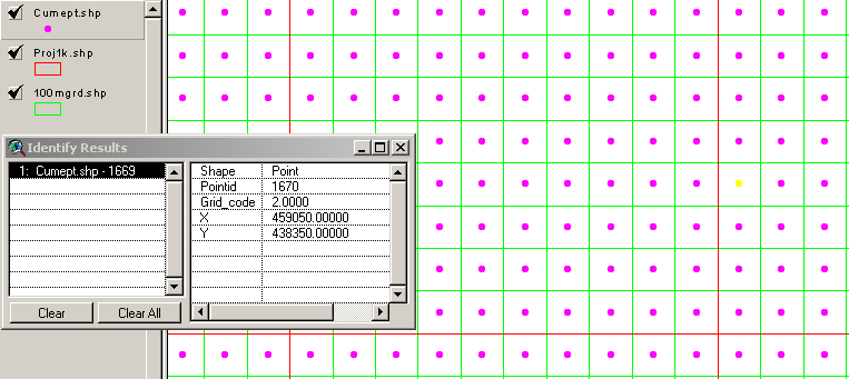
Figure 10: ArcView screen grab showing the point data as created by Grid Machine. The Grid_Code field shows the ADI value
Each of these point themes was then exported into an Access database, where they were merged into one table, based on a common ID field, which was created automatically during the conversion. The result was an Access table which contained all the appropriate information - an ID field and the value for each ADI in a separate field (Figure 11).
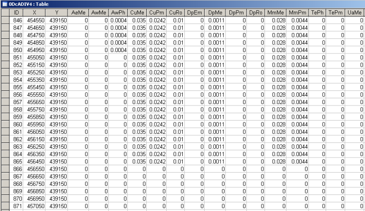
Figure 11: Example data from the Access table showing the various ADI fields with their associated data
This table was exported from Access as Dbase V file and it was possible to bring the Dbase V file back into ArcView and link it to the Shape File DCADIV4, using the Join command, as shown in Figure 12.
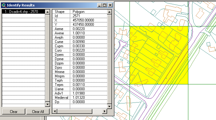
Figure 12: ArcView Screen grab showing the DCADIV4 data for the highlighted 100 metre square. Crown Copyright North Yorkshire County Council Licence No. 100017946 (2005)
© Internet Archaeology
URL: http://intarch.ac.uk/journal/issue21/1/3.html
Last updated: Wed April 25 2007